Tabulated proton and neutron densities
This notebook demonstrates the packaged density tables exposed through jitr.utils.density. The tables provide proton and neutron densities for specific (A, Z) targets in two density models, which can be interpolated onto any radial grid.
The densitiea are predictions of the deformed density distribution obtained within the Hartree-Fock-Bogoliubov method with the D1S Gogny effective interaction from
J. Decharge and D. Gogny, Phys. Rev. C21, 1568 (1980),
S. Hilaire and M. Girod, Eur. Phys. J. A33, 237 (2007),
and within the bskg3 Skyrme force:
S. Goriely, M. Samyn, and J.M. Pearson, Phys. Rev. C75, 064312 (2007),
G. Audi, A.H. Wapstra, and C. Thibault, Nucl. Phys. A729, 337 (2003),
I. Angeli, At. Data Nucl. Data Tables 87, 185 (2004).
The tables are copied from the TALYS code.
1import matplotlib.pyplot as plt
2import numpy as np
3
4from jitr.utils import density
5from jitr.utils.density import TwoParameterFermiDensity
1density.density_models()
['bskg3', 'd1m']
1density.density_models(), density.density_targets(model="d1m", Z=8)
(['bskg3', 'd1m'],
 [(12, 8),
  (13, 8),
  (14, 8),
  (15, 8),
  (16, 8),
  (17, 8),
  (18, 8),
  (19, 8),
  (20, 8),
  (21, 8),
  (22, 8),
  (23, 8),
  (24, 8),
  (25, 8),
  (26, 8),
  (27, 8),
  (28, 8),
  (29, 8),
  (30, 8)])
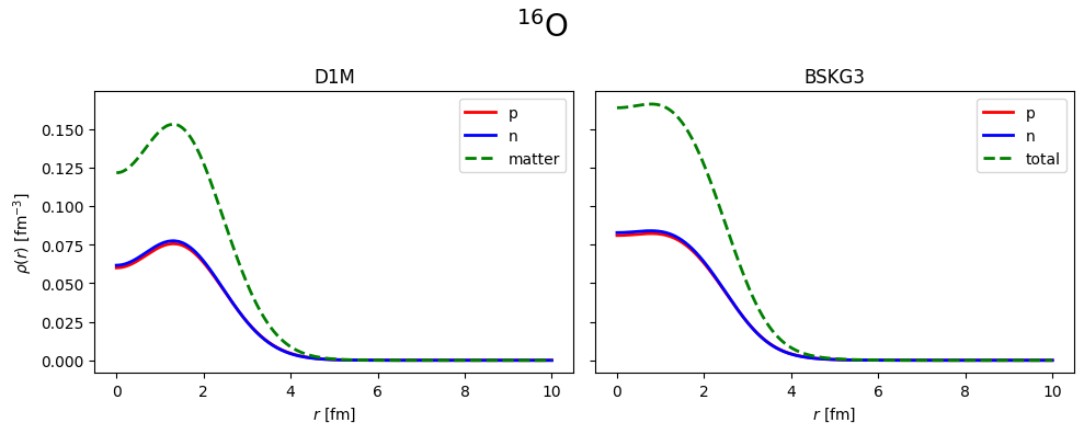
 1A, Z = 16, 8
 2r = np.linspace(0.0, 10.0, 400)
 3
 4rho_p_d1m, rho_n_d1m = density.densities(A, Z, r, model="d1m")
 5rho_p_bskg3, rho_n_bskg3 = density.densities(A, Z, r, model="bskg3")
 6
 7table = density.density_table(A, Z, model="d1m")
 8proton_number = (
 9    4.0
10    * np.pi
11    * np.trapezoid(
12        table.radial_grid**2 * table.proton_density_grid,
13        table.radial_grid,
14    )
15)
16neutron_number = (
17    4.0
18    * np.pi
19    * np.trapezoid(
20        table.radial_grid**2 * table.neutron_density_grid,
21        table.radial_grid,
22    )
23)
24
25assert np.isclose(proton_number, Z, rtol=1e-4)
26assert np.isclose(neutron_number, A - Z, rtol=1e-4)
 1fig, axes = plt.subplots(1, 2, figsize=(10, 4), sharey=True)
 2
 3axes[0].plot(r, rho_p_d1m, color="r", label="p", linewidth=2)
 4axes[0].plot(r, rho_n_d1m, color="b", label="n", linewidth=2)
 5axes[0].plot(
 6    r, rho_p_d1m + rho_n_d1m, color="g", label="matter", linestyle="--", linewidth=2
 7)
 8axes[0].set_title("D1M")
 9axes[0].set_xlabel(r"$r$ [fm]")
10axes[0].set_ylabel(r"$\rho(r)$ [fm$^{-3}$]")
11axes[0].legend()
12
13axes[1].plot(r, rho_p_bskg3, color="r", label="p", linewidth=2)
14axes[1].plot(r, rho_n_bskg3, color="b", label="n", linewidth=2)
15axes[1].plot(
16    r, rho_p_bskg3 + rho_n_bskg3, color="g", label="total", linestyle="--", linewidth=2
17)
18axes[1].set_title("BSKG3")
19axes[1].set_xlabel(r"$r$ [fm]")
20axes[1].legend()
21
22fig.suptitle(r"$^{16}$O", fontsize=20)
23fig.tight_layout()
1def pb208_densities_2pf():
2    rho_n = TwoParameterFermiDensity(R=6.6, a=0.55, N=126)
3    rho_p = TwoParameterFermiDensity(R=6.3, a=0.547, N=82)
4    return rho_p, rho_n
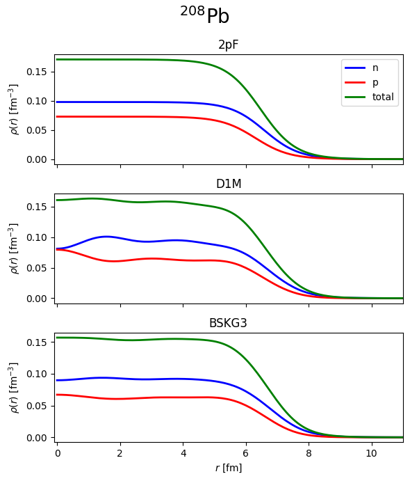
1def norm_and_rms_radii(rho, R):
2    m0 = 4 * np.pi * np.trapezoid(rho * R**2, R)
3    m2 = 4 * np.pi * np.trapezoid(rho * R**4, R)
4    return m0, np.sqrt(m2 / m0)
 1def print_density_stats(rho_p, rho_n, R):
 2    N, rms_n = norm_and_rms_radii(rho_n, R)
 3    Z, rms_p = norm_and_rms_radii(rho_p, R)
 4    Z, rms_m = norm_and_rms_radii(rho_p + rho_n, R)
 5    print(f"N: {N:1.2f}")
 6    print(f"Z: {Z:1.2f}")
 7    print(f"rms_n: {rms_n:1.2f} fm")
 8    print(f"rms_p: {rms_p:1.2f} fm")
 9    print(f"rms_m: {rms_m:1.2f} fm")
10    print(f"nskin: {rms_n - rms_p:1.3f} fm")
11
12
13def plot_densities(ax, rho_p, rho_n, R):
14    ax.plot(R, rho_n, color="b", label="n", linewidth=2)
15    ax.plot(R, rho_p, color="r", label="p", linewidth=2)
16    ax.plot(R, rho_n + rho_p, color="g", label="total", linewidth=2)
 1R = np.linspace(0.0, 15.0, 201)
 2rho_p_2pf, rho_n_2pf = pb208_densities_2pf()
 3rho_p_d1m, rho_n_d1m = density.densities(208, 82, R, model="d1m")
 4rho_p_bskg3, rho_n_bskg3 = density.densities(208, 82, R, model="bskg3")
 5print("208-Pb")
 6print("\n2pf:")
 7print("=======================")
 8print_density_stats(np.array(rho_p_2pf(R)), np.array(rho_n_2pf(R)), R)
 9
10print("\nd1m:")
11print("=======================")
12print_density_stats(rho_p_d1m, rho_n_d1m, R)
13
14print("\nbskg3")
15print("=======================")
16print_density_stats(rho_p_bskg3, rho_n_bskg3, R)
208-Pb

2pf:
=======================
N: 126.00
Z: 208.00
rms_n: 5.51 fm
rms_p: 5.29 fm
rms_m: 5.42 fm
nskin: 0.219 fm

d1m:
=======================
N: 126.00
Z: 208.00
rms_n: 5.58 fm
rms_p: 5.44 fm
rms_m: 5.52 fm
nskin: 0.131 fm

bskg3
=======================
N: 126.00
Z: 208.00
rms_n: 5.61 fm
rms_p: 5.45 fm
rms_m: 5.54 fm
nskin: 0.162 fm
 1fig, axes = plt.subplots(3, 1, figsize=(6, 7), sharex=True)
 2fig.suptitle(r"$^{208}$Pb", fontsize=20)
 3plot_densities(axes[0], np.array(rho_p_2pf(R)), np.array(rho_n_2pf(R)), R)
 4plot_densities(axes[1], rho_p_d1m, rho_n_d1m, R)
 5plot_densities(axes[2], rho_p_bskg3, rho_n_bskg3, R)
 6
 7axes[0].legend()
 8axes[2].set_xlabel(r"$r$ [fm]")
 9
10axes[0].set_ylabel(r"$\rho(r)$ [fm$^{-3}$]")
11axes[1].set_ylabel(r"$\rho(r)$ [fm$^{-3}$]")
12axes[2].set_ylabel(r"$\rho(r)$ [fm$^{-3}$]")
13
14axes[0].set_title(r"2pF")
15axes[1].set_title(r"D1M")
16axes[2].set_title(r"BSKG3")
17
18axes[0].set_xlim([-0.1, 11])
19plt.tight_layout()
20plt.show()