Dispersive optical model interface

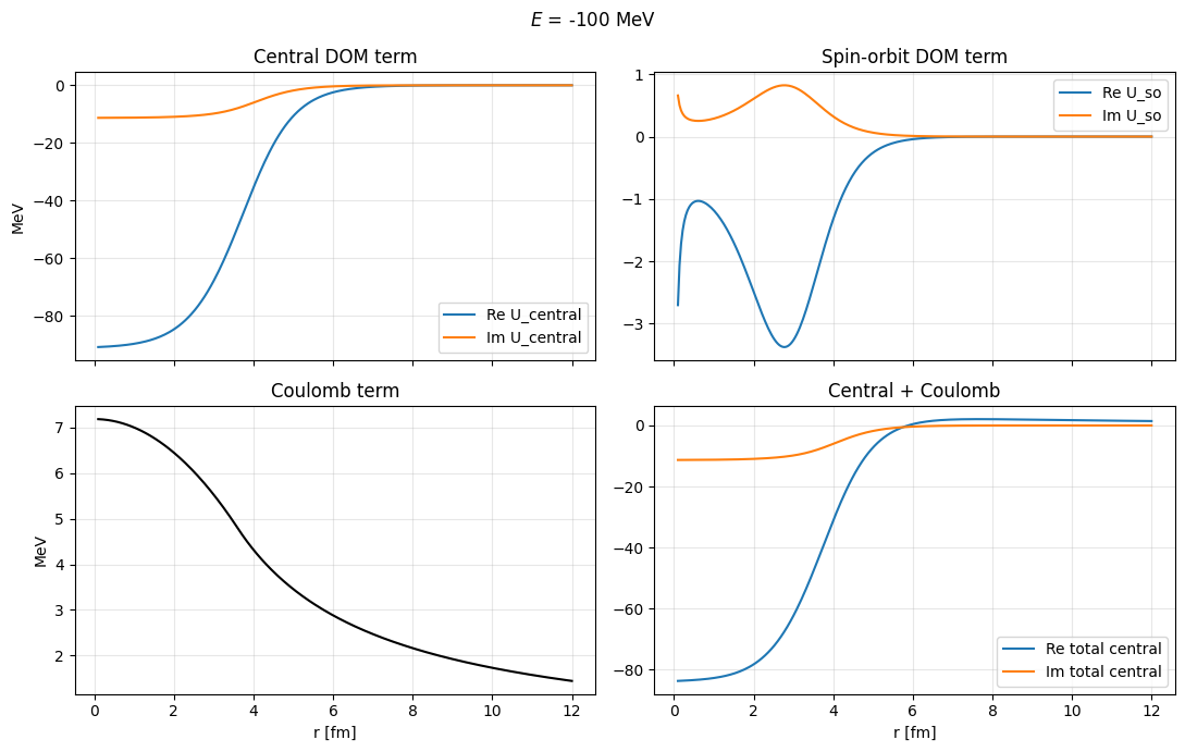
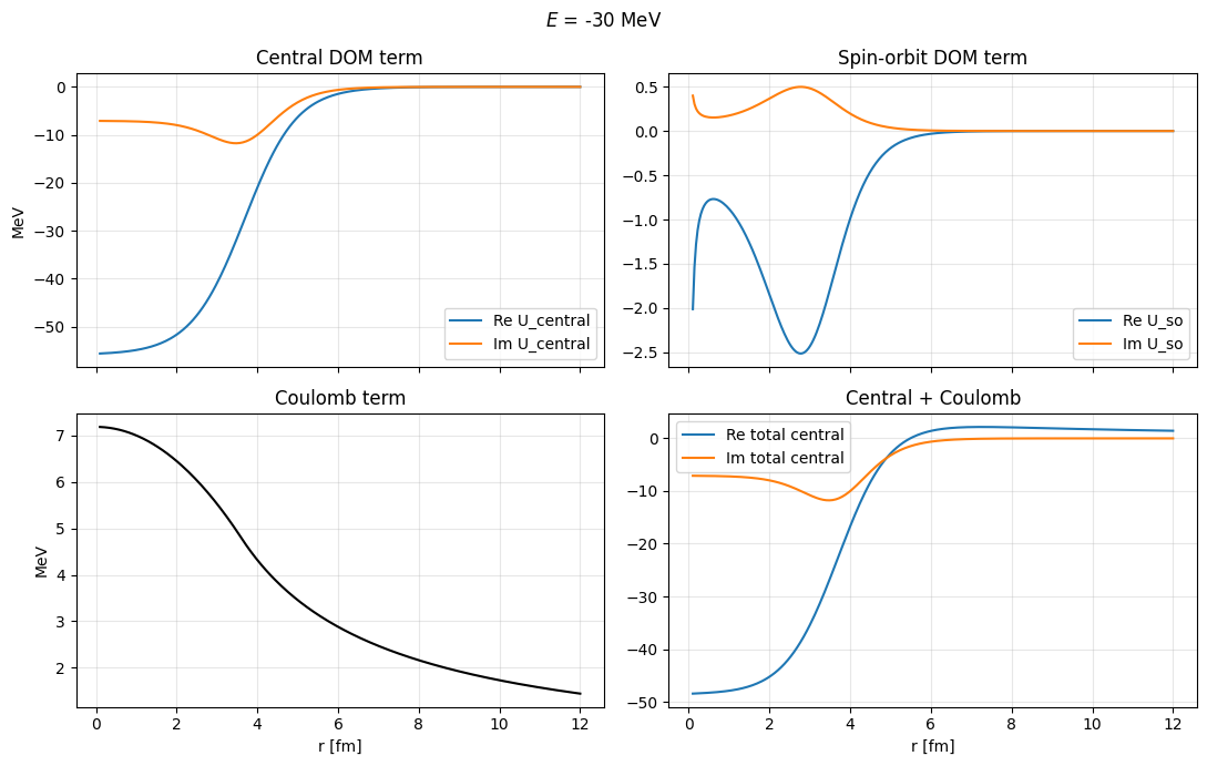
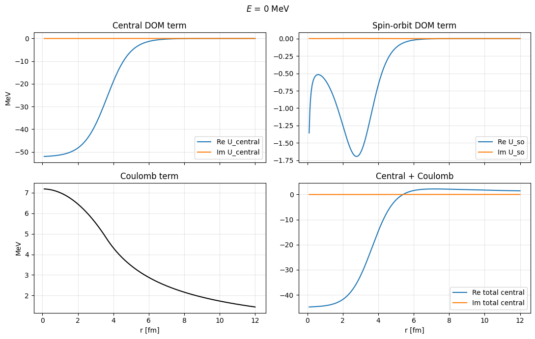
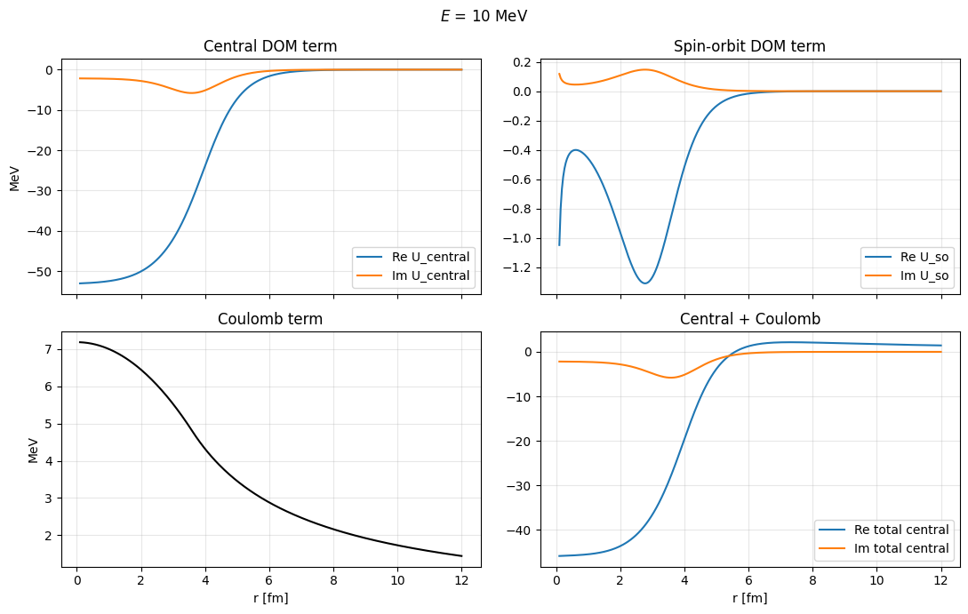
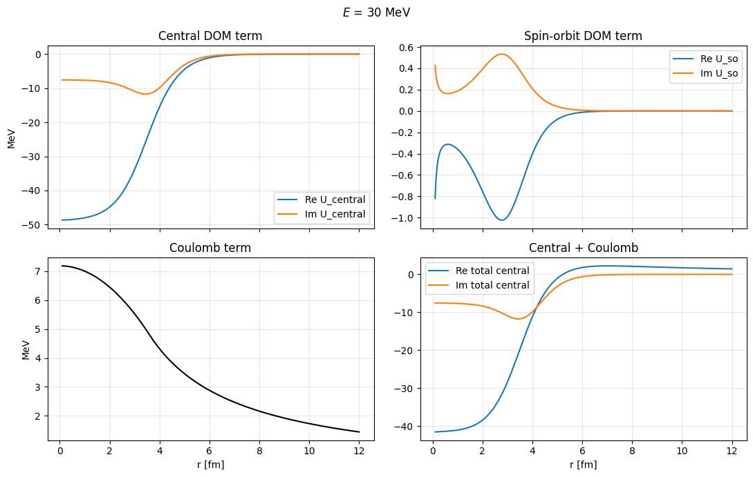
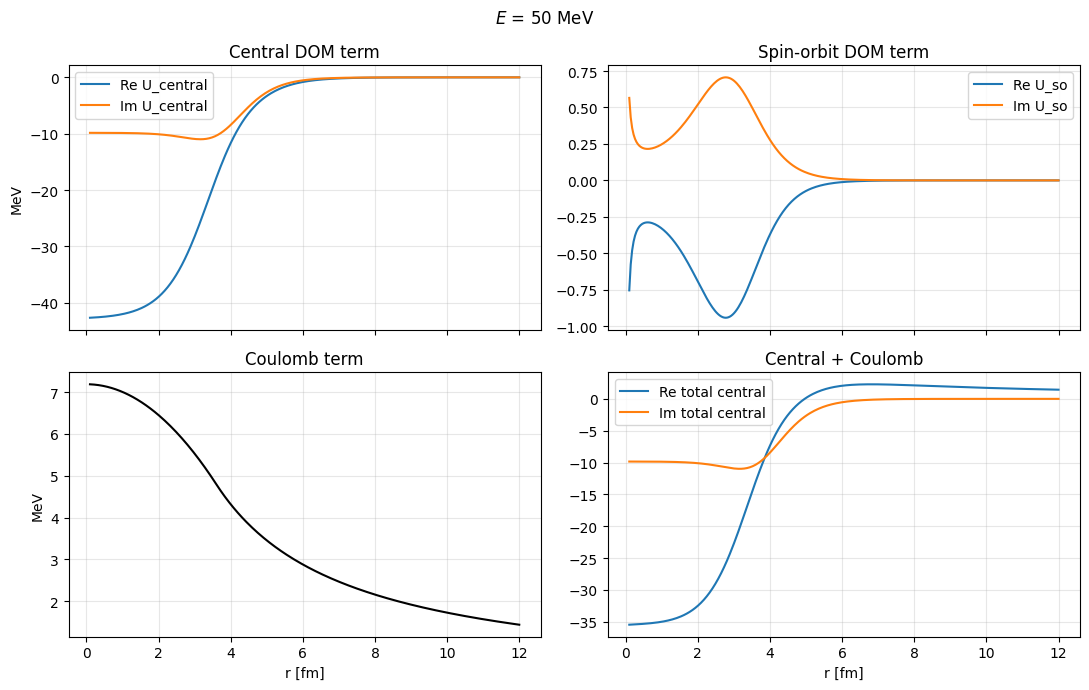
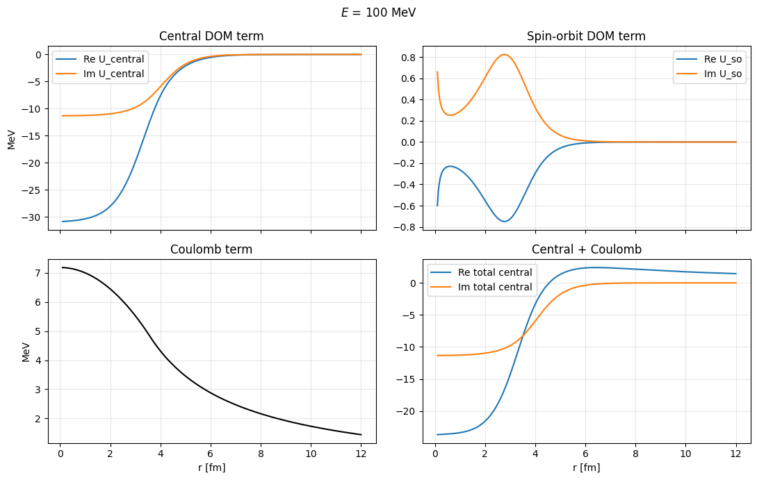
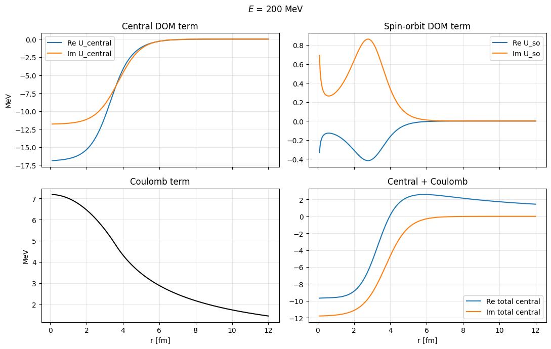
This notebook demonstrates the supported jitr.optical_potentials.dom interface. For a given parameter set, we plot the potential curves \(U(r)\) at multiple different energies.

import numpy as np
from matplotlib import pyplot as plt

from jitr.optical_potentials import dom
from jitr.reactions import ElasticReaction
from jitr.utils.kinematics import classical_kinematics_cm

params = {
    "v0": 52.0,
    "v1": 0.006,
    "rv": 1.25,
    "av": 0.65,
    "wv0": 12.0,
    "wv1": 24.0,
    "rw": 1.28,
    "aw": 0.62,
    "ws0": 15.0,
    "ws1": 12.5,
    "ws2": 0.021,
    "rd": 1.28,
    "ad": 0.55,
    "vso0": 6.0,
    "wso0": -3,
    "wso1": 25.0,
    "rso": 1.05,
    "aso": 0.59,
    "rC": 1.25,
}

model = dom.DOM()
param_names = model.params
param_values = [params[name] for name in param_names]
param_names

['v0',
 'v1',
 'rv',
 'av',
 'wv0',
 'wv1',
 'rw',
 'aw',
 'ws0',
 'ws1',
 'ws2',
 'rd',
 'ad',
 'vso0',
 'wso0',
 'wso1',
 'rso',
 'aso',
 'rC']

reaction = ElasticReaction((24, 12), (1, 1))
r_grid = np.linspace(0.1, 12.0, 300)

for E in [-100, -30, 0, 10, 30, 50, 100, 200]:
    kinematics = classical_kinematics_cm(
        reaction.target.m0,
        reaction.projectile.m0,
        Ecm=E,
        Zz=reaction.target.Z * reaction.projectile.Z,
    )

    U_central, U_spin_orbit, U_coulomb = model(
        r_grid, reaction, kinematics, *param_values
    )

    fig, axes = plt.subplots(2, 2, figsize=(11, 7), sharex=True)
    fig.suptitle(f"$E$ = {E} MeV")

    axes[0, 0].plot(r_grid, U_central.real, label="Re U_central")
    axes[0, 0].plot(r_grid, U_central.imag, label="Im U_central")
    axes[0, 0].set_ylabel("MeV")
    axes[0, 0].set_title("Central DOM term")
    axes[0, 0].legend()
    axes[0, 0].grid(alpha=0.3)

    axes[0, 1].plot(r_grid, U_spin_orbit.real, label="Re U_so")
    axes[0, 1].plot(r_grid, U_spin_orbit.imag, label="Im U_so")
    axes[0, 1].set_title("Spin-orbit DOM term")
    axes[0, 1].legend()
    axes[0, 1].grid(alpha=0.3)

    axes[1, 0].plot(r_grid, U_coulomb, color="black")
    axes[1, 0].set_xlabel("r [fm]")
    axes[1, 0].set_ylabel("MeV")
    axes[1, 0].set_title("Coulomb term")
    axes[1, 0].grid(alpha=0.3)

    axes[1, 1].plot(r_grid, (U_central + U_coulomb).real, label="Re total central")
    axes[1, 1].plot(r_grid, (U_central + U_coulomb).imag, label="Im total central")
    axes[1, 1].set_xlabel("r [fm]")
    axes[1, 1].set_title("Central + Coulomb")
    axes[1, 1].legend()
    axes[1, 1].grid(alpha=0.3)

    fig.tight_layout()