Elastic scattering with LocalOpticalPotential

LocalOpticalPotential provides a useful interface for defining optical potentials.

import numpy as np
from matplotlib import pyplot as plt
from pandas import DataFrame
from tqdm import tqdm

from jitr.optical_potentials import LocalOpticalPotential
from jitr.reactions.reaction import Reaction
from jitr.rmatrix import Solver as SolverKernel
from jitr.utils import utils
from jitr.xs import elastic

neutron = (1, 0)
proton = (1, 1)

target = (208, 82)
projectile = proton
energy_lab = 24
reaction = Reaction(target=target, projectile=projectile, process="El")
kinematics = reaction.kinematics(energy_lab)

# set the channel radius, number of nodes, and number of partial waves
interaction_range_fm = 1.2 * (208 ** (1 / 3)) + 1
channel_radius_dimensionless = utils.suggested_dimensionless_channel_radius(
    interaction_range_fm, kinematics.k
)
channel_radius = channel_radius_dimensionless / kinematics.k
N = utils.suggested_basis_size(channel_radius_dimensionless)
lmax = 50

# build a solver for the system and reaction of interest
print(f"Compiling solver for {reaction} at {energy_lab} MeV")
print(f" - channel radius {channel_radius:1.2f} fm")
print(f" - {N} nodes")
print(f" - {lmax} partial waves")

solver = elastic.DifferentialWorkspace.build_from_system(
    reaction=reaction,
    kinematics=kinematics,
    channel_radius_fm=channel_radius,
    solver=SolverKernel(N),
    lmax=lmax,
    angles=np.linspace(0.1, np.pi, 180),
)
rgrid = solver.radial_grid()
print("Done!")

Compiling solver for 208-Pb(p,el) at 24 MeV
 - channel radius 13.94 fm
 - 25 nodes
 - 50 partial waves
Done!

Use the built-in LocalOpticalPotential class

Although, in general, one can define whatever interaction they want. This is just a handy tool.

omp = LocalOpticalPotential()
omp.params

['Vv',
 'rv',
 'av',
 'Wv',
 'rw',
 'aw',
 'Wd',
 'Vd',
 'rd',
 'ad',
 'Vso',
 'Wso',
 'rso',
 'aso',
 'rC']

Randomly generate a bunch of parameters

means = np.array([56, 1.2, 0.7, 5, 1.2, 0.7, 13, 6, 1.3, 0.9, 8, 4, 1.1, 0.7, 1.2])
std_devs = np.array(
    [3, 0.05, 0.03, 0.1, 0.05, 0.05, 1, 0.1, 0.1, 0.1, 0.2, 1, 0.1, 0.05, 0.1]
)
samples = np.random.multivariate_normal(means, np.diag(std_devs) ** 2, 1000)

df = DataFrame(samples, columns=omp.params)
df.head()

	Vv	rv	av	Wv	rw	aw	Wd	Vd	rd	ad	Vso	Wso	rso	aso	rC
0	51.100403	1.193229	0.694053	5.001168	1.204845	0.698625	11.593592	6.002358	1.180502	0.987147	8.170491	3.076880	1.085694	0.734179	1.339886
1	52.833976	1.219670	0.686945	4.859437	1.260052	0.711278	11.806969	5.940825	1.241372	0.904550	8.085328	4.380284	1.151938	0.721191	1.342671
2	60.490654	1.111695	0.690334	5.017723	1.266576	0.709783	11.567632	6.207810	1.380022	0.802054	8.088928	3.947422	1.042329	0.771521	1.315199
3	55.871365	1.194629	0.746419	5.118907	1.167164	0.682690	13.338335	6.052000	1.309950	0.599037	7.906294	4.470666	1.194999	0.675212	1.157940
4	55.460503	1.117543	0.733219	4.896455	1.210000	0.658962	14.617597	6.307500	1.341588	0.890594	8.172465	4.120561	1.102040	0.620034	1.185585

How do we calculate observables?

We are using a jitr.xs.elastic.DifferentialWorkspace, which is set up specifically to interface with omp and other classes that have the same structure

help(elastic.DifferentialWorkspace.xs)

Help on function xs in module jitr.xs.elastic:

xs(self, central_potential: 'npt.ArrayLike', spin_orbit_potential: 'npt.ArrayLike | None' = None, coulomb_potential: 'npt.ArrayLike | None' = None) -> 'ElasticXS'
    Return differential and integral elastic observables.

Exactly the information that the solver workspace needs is what is provided by the omp class:

help(omp.evaluate)

Help on method evaluate in module jitr.optical_potentials.omp:

evaluate(rgrid: 'ArrayOrScalar', reaction_model: 'reaction.Reaction', kinematics_model: 'kinematics.ChannelKinematics', Vv: 'float', rv: 'float', av: 'float', Wv: 'float', rw: 'float', aw: 'float', Wd: 'float', Vd: 'float', rd: 'float', ad: 'float', Vso: 'float', Wso: 'float', rso: 'float', aso: 'float', rC: 'float') -> 'tuple[PotentialArray, PotentialArray, PotentialArray | ArrayOrScalar]' method of jitr.optical_potentials.omp.LocalOpticalPotential instance
    Evaluate the local optical-potential terms on ``rgrid``.

Do you see the vision?

Now running calculations is simple! Once it’s been compiled, it’s fast:

%%time
num_samples, num_params = df.shape
xs_ratio = np.zeros((num_samples, solver.angles.size))
Ay = np.zeros((num_samples, solver.angles.size))
rgrid = solver.radial_grid()

for i in tqdm(range(num_samples)):
    central_term, spin_orbit_term, coulomb_term = omp(
        rgrid,
        reaction,
        kinematics,
        *samples[i, :],
    )
    xs = solver.xs(central_term, spin_orbit_term, coulomb_term)
    xs_ratio[i, :] = xs.dsdo / solver.rutherford
    Ay[i, :] = xs.Ay

100%|██████████████████████████████████████████████████████████| 1000/1000 [00:09<00:00, 100.51it/s]

CPU times: user 9.68 s, sys: 265 ms, total: 9.94 s
Wall time: 9.95 s

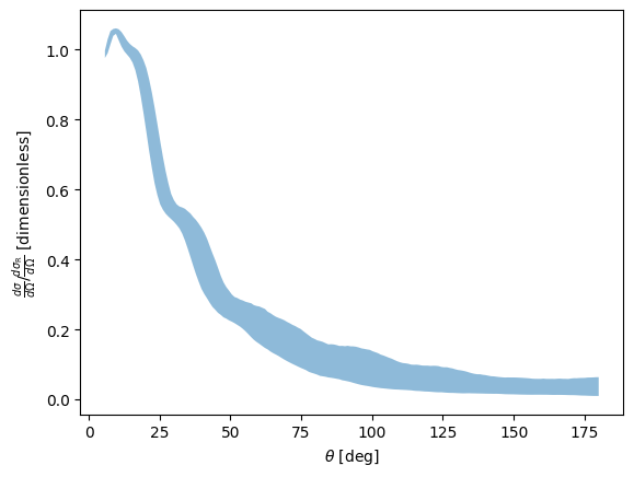
plt.fill_between(
    np.rad2deg(solver.angles), *np.percentile(xs_ratio, [5, 95], axis=0), alpha=0.5
)
plt.xlabel(r"$\theta$ [deg]")
plt.ylabel(
    r"$\frac{d \sigma}{d\Omega} / \frac{d \sigma_{\text{R}}}{d\Omega}$ [dimensionless]"
)

Text(0, 0.5, '$\\frac{d \\sigma}{d\\Omega} / \\frac{d \\sigma_{\\text{R}}}{d\\Omega}$ [dimensionless]')

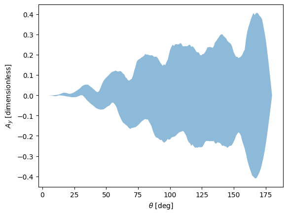
plt.fill_between(
    np.rad2deg(solver.angles), *np.percentile(Ay, [5, 95], axis=0), alpha=0.5
)
plt.xlabel(r"$\theta$ [deg]")
plt.ylabel(r"$A_y$ [dimensionless]")

Text(0, 0.5, '$A_y$ [dimensionless]')