JLM and JLMB semi-microscopic optical potentials
1import matplotlib as mpl
2import matplotlib.pyplot as plt
3import numpy as np
1from jitr.folding import ILDAFolder, jlm
2from jitr.utils import density
3from jitr.utils.density import TwoParameterFermiDensity
Optical potential from nuclear matter
The JLM (for J. P. Jeukenne, A. Lejeune, and C. Mahaux) model for the nuclear matter self-energy is included in jitr, as defined in the seminal works JLM, 1974, JLM, 1977a, and JLM, 1977b.
The goal was to try to model the effective interactions (optical potential) nucleons feel in when scattering on a nucleus by treating the many-body dynamics as if that nucleon where interacting with a system of homogenous nuclear matter, at the local local density of its position withion the medium of the finite nucleus. This work takes multiple steps:
Calculate the nuclear matter self energy at various matter densities \(\rho\) and nucleon energies \(E\): \(\Sigma(\rho,E)\)
determine a model for the density distribution of a finite nucleus \(\rho(r)\)
Evaluate the optical potential for the finite nucleus in the local density approximation: \(\Sigma(r,E) = \Sigma(\rho(r),E)\)
Later, E. Bauge, J. P. Delaroche, and M. Girod updated this JLM microscopic optical potential in various ways, including adjusting the energy dependence to fit to scattering data (See BDG 1998 and BDG, 2001). This is known as the JLMB semi-microscopic optical potential, and it is included in the reaction code TALYS, which is used for nuclear data evaluation.
In this notebook, we will describe both of these models, and demonstrate their implementation in jitr.
The nuclear matter self energy
The nuclear matter self energy is determined from Brueckner-Hartree Fock (BHF) calculations of the \(g\)-matrix in symmetric nuclear matter and nuclear matter with neutron excess, using Reid’s hard core interaction, at various matter densities (Fermi momenta) and a range of positive energies from 10 to 160 MeV, producing isoscalar and isovector effective 2-body interactions. By contracting these two-body interactions over the occupied states in nuclear matter, one determines the nuclear matter self-energy felt by a single nucleon. This self energy can be decomposed into isoscalar and isovector terms:
with \(\alpha = (\rho_n - \rho_p) / (\rho_n + \rho_p)\), and the \(+(-)\) sign for neutrons(protons).
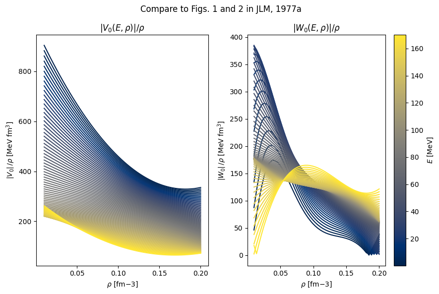
The isoscalar real self energy, \(V_0(\rho,E)\) was parameterized as a polynomial fit to the BHF results:
The isoscalar imaginary part \(W_0(\rho,E)\) was parameterized as
with \(D=600\) and the Fermi energy parameterized from the Brueckner-Hartree-Fock result as:
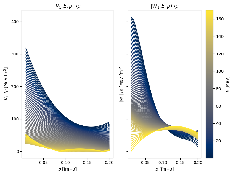
The isovector real and imaginary parts are respectively defined as
where \(N(\rho,E)\) is extracted from the Coulomb-corrected difference of the neutron and proton self-energies in nuclear matter, with a given neutron excess (See JLM, 1977b). \(N\) is parameterized as:
with \(F=1\). The \(k\)-mass, \(\tilde{m}(\rho,E)\) is parameterized as
The \(E\)-mass \(\bar{m}(\rho,E)\) can be obtained from
where the effective mass is defined
In total, there are 5 coefficient matrices, \(a\), \(b\), \(c\), \(d\), \(f\).
These are included in jitr.folding.jlm.
1rho_sat_fm3 = 0.16
1jlm.fermi_energy_MeV(rho_sat_fm3)
np.float64(-24.844800000000003)
Note that the BHF calculation using Reid’s hard core interaction do not preduce the empirical saturation in nuclear matter.
1rho_grid = np.linspace(0.01, 0.2, 50)
2E_vals = np.linspace(0.1, 170, 80)
 1fig, axes = plt.subplots(1, 2, figsize=(9, 6), sharey=False)
 2cmap = plt.cm.cividis
 3norm = mpl.colors.Normalize(vmin=E_vals.min(), vmax=E_vals.max())
 4E_F = jlm.fermi_energy_MeV(rho_grid)
 5for E in E_vals:
 6    axes[0].plot(
 7        rho_grid,
 8        np.abs(jlm.V0(rho_grid, E)) / rho_grid,
 9        color=cmap(norm(E)),
10        label=f"{E:1.0f} MeV",
11    )
12    axes[1].plot(
13        rho_grid,
14        np.abs(jlm.W0(rho_grid, E, E_F=E_F)) / rho_grid,
15        label=f"{E:1.0f} MeV",
16        color=cmap(norm(E)),
17    )
18
19axes[0].set_title(r"$|V_0(E,\rho)| / \rho$")
20axes[0].set_ylabel(r"$|V_0 | \, / \rho $ [MeV fm$^3$]")
21axes[0].set_xlabel(r"$\rho$ [fm${-3}$]")
22
23axes[1].set_title(r"$|W_0(E,\rho)| / \rho$")
24axes[1].set_xlabel(r"$\rho$ [fm${-3}$]")
25axes[1].set_ylabel(r"$|W_0 | \, / \rho $ [MeV fm$^3$]")
26# axes[1].legend()
27
28
29sm = mpl.cm.ScalarMappable(norm=norm, cmap=cmap)
30sm.set_array([])
31
32cbar = fig.colorbar(sm, ax=axes[1])
33cbar.set_label("$E$ [MeV]")
34
35fig.suptitle("Compare to Figs. 1 and 2 in JLM, 1977a")
36
37plt.tight_layout()
38plt.show()
 1fig, axes = plt.subplots(1, 2, figsize=(8, 6), sharey=True)
 2E_F = jlm.fermi_energy_MeV(rho_grid)
 3for E in E_vals:
 4    axes[0].plot(
 5        rho_grid,
 6        np.abs(jlm.V1(rho_grid, E, E_F=E_F)) / rho_grid,
 7        color=cmap(norm(E)),
 8        label=f"{E:1.0f} MeV",
 9    )
10    axes[1].plot(
11        rho_grid,
12        np.abs(jlm.W1(rho_grid, E, E_F=E_F)) / rho_grid,
13        label=f"{E:1.0f} MeV",
14        color=cmap(norm(E)),
15    )
16
17axes[0].set_title(r"$|V_1(E,\rho)| / \rho$")
18axes[0].set_ylabel(r"$|V_1 | \, / \rho $ [MeV fm$^3$]")
19axes[0].set_xlabel(r"$\rho$ [fm${-3}$]")
20
21axes[1].set_title(r"$|W_1(E,\rho)| / \rho$")
22axes[1].set_xlabel(r"$\rho$ [fm${-3}$]")
23axes[1].set_ylabel(r"$|W_1 | \, / \rho $ [MeV fm$^3$]")
24# axes[1].legend()
25sm = mpl.cm.ScalarMappable(norm=norm, cmap=cmap)
26sm.set_array([])
27
28cbar = fig.colorbar(sm, ax=axes[1])
29cbar.set_label("$E$ [MeV]")
30
31
32plt.tight_layout()
33plt.show()
Folding to finite nuclear density
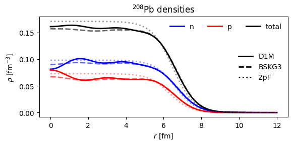
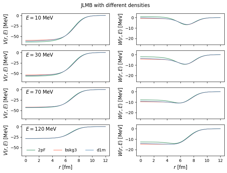
We will use the local density approximation and improved local density approximations. First, let’s grab some density distributions:
1def pb208_densities_2pf():
2    rho_n = TwoParameterFermiDensity(R=6.6, a=0.55, N=126)
3    rho_p = TwoParameterFermiDensity(R=6.3, a=0.547, N=82)
4    return rho_p, rho_n
1target = (208, 82)
2neutron = (1, 0)
3proton = (1, 1)
4
5R = np.linspace(0.0, 12.0, 201)
6
7rho_p_2pf, rho_n_2pf = pb208_densities_2pf()
8rho_p_d1m, rho_n_d1m = density.densities(208, 82, R, model="d1m")
9rho_p_bskg3, rho_n_bskg3 = density.densities(208, 82, R, model="bskg3")
 1fig, ax = plt.subplots(figsize=(6, 3))
 2legend_handles_density_type = [
 3    ax.plot(R, rho_n_d1m, color="b", label="n", linewidth=2)[0],
 4    ax.plot(R, rho_p_d1m, color="r", label="p", linewidth=2)[0],
 5    ax.plot(R, rho_n_d1m + rho_p_d1m, color="k", label="total", linewidth=2)[0],
 6]
 7
 8plt.plot(R, rho_n_bskg3, "--", color="b", linewidth=2, alpha=0.6)
 9plt.plot(R, rho_p_bskg3, "--", color="r", linewidth=2, alpha=0.6)
10plt.plot(R, rho_n_bskg3 + rho_p_bskg3, "--", color="k", linewidth=2, alpha=0.6)
11
12
13plt.plot(R, rho_n_2pf(R), ":", color="b", linewidth=2, alpha=0.4)
14plt.plot(R, rho_p_2pf(R), ":", color="r", linewidth=2, alpha=0.4)
15plt.plot(R, rho_n_2pf(R) + rho_p_2pf(R), ":", color="k", linewidth=2, alpha=0.4)
16
17leg1 = ax.legend(
18    handles=legend_handles_density_type, framealpha=0, ncol=3, loc="upper right"
19)
20leg2 = plt.legend(
21    handles=[
22        plt.plot([], [], color="k", linewidth=2, label="D1M")[0],
23        plt.plot([], [], "--", color="k", linewidth=2, label="BSKG3")[0],
24        plt.plot([], [], ":", color="k", linewidth=2, label="2pF")[0],
25    ],
26    framealpha=0,
27    loc="center right",
28)
29
30ax.add_artist(leg1)
31
32plt.xlabel(r"$r$ [fm]")
33plt.ylabel(r"$\rho$ [fm$^{-3}$]")
34plt.title(r"$^{208}$Pb densities")
35plt.tight_layout()
36plt.show()
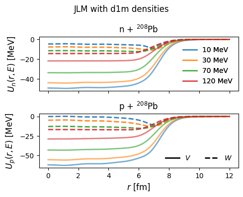
Local density approximation (LDA)
The LDA is a simple prescription. Given a nuclear matter self-energy \(U(\rho,E)\) and a density profile \(\rho(r)\):
From JLM, 1977b:
[the] local density approximation (LDA) ascribes to the OMP at the density \(\rho(r)\) the same value as in a uniform medium with the same value of the density, with the same neutron excess, and at the same energy.
 1fig, axes = plt.subplots(2, 1, sharex=True, figsize=(5, 4))
 2handles_energy = []
 3folder_local = ILDAFolder(r_max=20.0, n_quad=200)
 4V_C_local = folder_local.V_coulomb(
 5    folder_local.interp_to_quad(R, rho_p_d1m),
 6    mode="density",
 7    include_exchange=True,
 8    r_out=R,
 9)
10for E in [10, 30, 70, 120]:
11    V, W = jlm.potential_JLM(R, rho_n_d1m + rho_p_d1m, (1, 0), target, E)
12    (p,) = axes[0].plot(R, V, linewidth=2, label=f"{E:1.0f} MeV", alpha=0.6)
13    axes[0].plot(R, W, "--", linewidth=2, color=p.get_color(), alpha=0.9)
14    handles_energy.append(p)
15    V, W = jlm.potential_JLM(
16        R,
17        rho_n_d1m + rho_p_d1m,
18        (1, 1),
19        target,
20        E,
21        V_C=V_C_local,
22        parameterization="talys",
23    )
24    axes[1].plot(R, V, linewidth=2, color=p.get_color(), alpha=0.6)
25    axes[1].plot(R, W, "--", linewidth=2, color=p.get_color(), alpha=0.9)
26
27leg1 = axes[0].legend(handles=handles_energy, framealpha=0, ncol=1, loc="lower right")
28leg2 = axes[1].legend(
29    handles=[
30        plt.plot([], [], color="k", linewidth=2, label=r"$V$")[0],
31        plt.plot([], [], "--", color="k", linewidth=2, label="$W$")[0],
32    ],
33    framealpha=0,
34    ncol=2,
35    loc="lower right",
36)
37axes[0].add_artist(leg1)
38
39
40axes[1].set_xlabel(r"$r$ [fm]", fontsize=12)
41axes[0].set_ylabel(r"$U_n(r,E)$ [MeV]", fontsize=12)
42axes[1].set_ylabel(r"$U_p(r,E)$ [MeV]", fontsize=12)
43axes[0].set_title(r"n + $^{208}$Pb", fontsize=12)
44axes[1].set_title(r"p + $^{208}$Pb", fontsize=12)
45fig.suptitle("JLM with d1m densities")
46plt.tight_layout()
47plt.show()
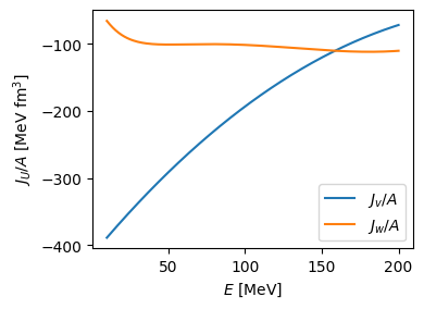
Volume integrals in the LDA
1energies = np.linspace(10, 200, 200)
2Ju_A = np.zeros_like(energies, dtype=complex)
3projectile = neutron
4A = target[0]
5for i, E in enumerate(energies):
6    V, W = jlm.potential_JLM(R, rho_n_d1m + rho_p_d1m, projectile, target, E)
7    Jv_A = 4 * np.pi / A * np.trapezoid(V * R**2, R)
8    Jw_A = 4 * np.pi / A * np.trapezoid(W * R**2, R)
9    Ju_A[i] = Jv_A + 1j * Jw_A
1fig = plt.figure(figsize=(4, 3))
2plt.plot(energies, Ju_A.real, label=r"$J_v/A$")
3plt.plot(energies, Ju_A.imag, label=r"$J_w/A$")
4plt.legend()
5plt.xlabel("$E$ [MeV]")
6plt.ylabel("$J_U / A$ [MeV fm$^3$]")
7plt.tight_layout()
8plt.show()
JLMB and the improved LDA (ILDA)
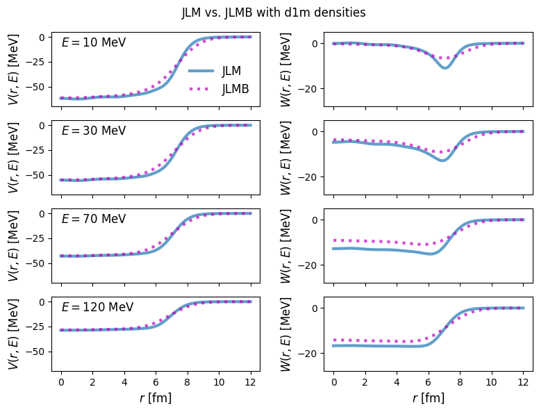
The JLM formalism was later updated to separately use the neutron and proton densities to determine the isovector dependence of the optical potential, as well renormalize the depths to fit elastic scattering experiments:
Additionally, rather than using the LDA as above, the finite nucleus self-energy as calculated above is convolved with a Gaussian with isovector-dependent range \(t \sim 1\) fm.
1folder = ILDAFolder(r_max=20.0, n_quad=200)  # once
2
3# interpolate densities onto quadrature g
4rho_n_q = folder.interp_to_quad(R, rho_n_d1m)
5rho_p_q = folder.interp_to_quad(R, rho_p_d1m)
 1energies = [10, 30, 70, 120]
 2projectile = proton
 3V_C_q = folder.V_coulomb(rho_p_q, mode="density", include_exchange=True)
 4V_C_R = folder.V_coulomb(rho_p_q, mode="density", include_exchange=True, r_out=R)
 5
 6fig, axes = plt.subplots(len(energies), 2, sharex=True, figsize=(8, 6))
 7axes = np.array(axes)
 8for i, E in enumerate(energies):
 9    V_n_jlm, W_n_jlm = jlm.potential_JLM(
10        R,
11        rho_n_d1m + rho_p_d1m,
12        projectile,
13        target,
14        E,
15        V_C=V_C_R,
16        parameterization="talys",
17    )
18    V_n_jlmb, W_n_jlmb = jlm.potential_JLMB(
19        folder,
20        rho_n_q,
21        rho_p_q,
22        projectile,
23        target,
24        E,
25        V_C=V_C_q,
26        parameterization="talys",
27        r_out=R,
28        lambda_V=jlm.lambda_v0(E),
29        lambda_V1=jlm.lambda_v1(E),
30        lambda_W=jlm.lambda_w0(E),
31        lambda_W1=jlm.lambda_w1(E),
32    )
33
34    axes[i, 0].plot(R, V_n_jlm, linewidth=3, alpha=0.7, color="tab:blue", label="JLM")
35    axes[i, 0].plot(R, V_n_jlmb, ":", linewidth=3, color="m", alpha=0.7, label="JLMB")
36    axes[i, 0].set_ylabel(r"$V(r,E)$ [MeV]", fontsize=12)
37    axes[i, 0].text(0, -10, f"$E = ${E:1.0f} MeV", fontsize=12)
38    axes[i, 0].set_ylim([-70, 5])
39
40    axes[i, 1].plot(R, W_n_jlm, linewidth=3, alpha=0.7, color="tab:blue", label="JLM")
41    axes[i, 1].plot(R, W_n_jlmb, ":", linewidth=3, color="m", alpha=0.7, label="JLMB")
42    axes[i, 1].set_ylabel(r"$W(r,E)$ [MeV]", fontsize=12)
43    axes[i, 1].set_ylim([-28, 5])
44
45
46axes[0, 0].legend(loc="lower right", framealpha=0, fontsize=12)
47axes[-1, 0].set_xlabel(r"$r$ [fm]", fontsize=12)
48axes[-1, 1].set_xlabel(r"$r$ [fm]", fontsize=12)
49fig.suptitle("JLM vs. JLMB with d1m densities")
50plt.tight_layout()
51plt.show()
 1energies = [10, 30, 70, 120]
 2projectile = proton
 3
 4# interpolate densities onto quadrature grid
 5densities_at_nodes = {
 6    label: (folder.interp_to_quad(R, rho_n), folder.interp_to_quad(R, rho_p))
 7    for label, rho_n, rho_p in [
 8        ("2pF", rho_n_2pf(R), rho_p_2pf(R)),
 9        ("bskg3", rho_n_bskg3, rho_p_bskg3),
10        ("d1m", rho_n_d1m, rho_p_d1m),
11    ]
12}
13
14colors = {
15    "2pF": "#2E8B57",
16    "d1m": "#4682B4",
17    "bskg3": "#FF6347",
18}
19
20fig, axes = plt.subplots(len(energies), 2, sharex=True, figsize=(8, 6))
21axes = np.array(axes)
22for i, E in enumerate(energies):
23    for model_name, (rho_n_q, rho_p_q) in densities_at_nodes.items():
24        V_C_q = folder.V_coulomb(rho_p_q, mode="density", include_exchange=True)
25        V, W = jlm.potential_JLMB(
26            folder,
27            rho_n_q,
28            rho_p_q,
29            projectile,
30            target,
31            E,
32            V_C=V_C_q,
33            parameterization="talys",
34            r_out=R,
35            lambda_V=jlm.lambda_v0(E),
36            lambda_V1=jlm.lambda_v1(E),
37            lambda_W=jlm.lambda_w0(E),
38            lambda_W1=jlm.lambda_w1(E),
39        )
40
41        axes[i, 0].plot(
42            R, V, linewidth=1, alpha=1, color=colors[model_name], label=model_name
43        )
44        axes[i, 1].plot(R, W, linewidth=1, alpha=1, color=colors[model_name])
45
46    axes[i, 0].set_ylabel(r"$V(r,E)$ [MeV]", fontsize=12)
47    axes[i, 0].text(0, -10, f"$E = ${E:1.0f} MeV", fontsize=12)
48    axes[i, 0].set_ylim([-70, 5])
49    axes[i, 1].set_ylabel(r"$W(r,E)$ [MeV]", fontsize=12)
50    axes[i, 1].set_ylim([-26, 4])
51
52
53axes[-1, 0].legend(loc="lower right", framealpha=0, fontsize=10, ncol=3)
54axes[-1, 0].set_xlabel(r"$r$ [fm]", fontsize=12)
55axes[-1, 1].set_xlabel(r"$r$ [fm]", fontsize=12)
56fig.suptitle("JLMB with different densities")
57plt.tight_layout()
58plt.show()
 1energies = np.linspace(0.01, 300, 200)
 2Ju_A_JLM = np.zeros_like(energies, dtype=complex)
 3Ju_A_JLMB = np.zeros_like(energies, dtype=complex)
 4Ju_A_JLMB_no_renorm = np.zeros_like(energies, dtype=complex)
 5
 6projectile = neutron
 7A = target[0]
 8for i, E in enumerate(energies):
 9    V, W = jlm.potential_JLM(R, rho_n_d1m + rho_p_d1m, projectile, target, E)
10    Ju_A_JLM[i] = np.trapezoid(V * R**2, R) + 1j * np.trapezoid(W * R**2, R)
11
12    V, W = jlm.potential_JLMB(
13        folder,
14        rho_n_q,
15        rho_p_q,
16        projectile,
17        target,
18        E,
19        lambda_V=jlm.lambda_v0(E),
20        lambda_V1=jlm.lambda_v1(E),
21        lambda_W=jlm.lambda_w0(E),
22        lambda_W1=jlm.lambda_w1(E),
23    )
24    Ju_A_JLMB[i] = folder.integrate(V * folder.r_q**2) + 1j * folder.integrate(
25        W * folder.r_q**2
26    )
27
28    V, W = jlm.potential_JLMB(
29        folder,
30        rho_n_q,
31        rho_p_q,
32        projectile,
33        target,
34        E,
35    )
36    Ju_A_JLMB_no_renorm[i] = folder.integrate(
37        V * folder.r_q**2
38    ) + 1j * folder.integrate(W * folder.r_q**2)
39
40Ju_A_JLM *= 4 * np.pi / A
41Ju_A_JLMB *= 4 * np.pi / A
42Ju_A_JLMB_no_renorm *= 4 * np.pi / A
 1fig, ax = plt.subplots(1, 1, figsize=(6, 4))
 2
 3legend_handles_term = [
 4    plt.plot(
 5        energies,
 6        Ju_A_JLM.real,
 7        linewidth=2,
 8        color="tab:blue",
 9        alpha=0.5,
10        label=r"$J_v/A$",
11    )[0],
12    plt.plot(
13        energies,
14        Ju_A_JLM.imag,
15        linewidth=2,
16        color="tab:orange",
17        alpha=0.5,
18        label=r"$J_w/A$",
19    )[0],
20]
21plt.plot(energies, Ju_A_JLMB.real, "--", linewidth=2, color="tab:blue")
22plt.plot(energies, Ju_A_JLMB.imag, "--", linewidth=2, color="tab:orange")
23plt.plot(energies, Ju_A_JLMB_no_renorm.real, ":", linewidth=2, color="tab:blue")
24plt.plot(energies, Ju_A_JLMB_no_renorm.imag, ":", linewidth=2, color="tab:orange")
25
26leg1 = ax.legend(
27    handles=legend_handles_term,
28    framealpha=0,
29    ncol=1,
30    loc="center",
31    fontsize=12,
32)
33leg2 = plt.legend(
34    handles=[
35        plt.plot([], [], color="k", linewidth=2, label="JLM")[0],
36        plt.plot([], [], "--", color="k", linewidth=2, label="JLMB")[0],
37        plt.plot([], [], ":", color="k", linewidth=2, label=r"JLMB, $\lambda_i = 1$")[
38            0
39        ],
40    ],
41    framealpha=0,
42    loc="center left",
43    fontsize=12,
44)
45ax.add_artist(leg1)
46
47
48plt.xscale("log")
49plt.xlabel("$E$ [MeV]", fontsize=12)
50plt.ylabel("$J_U / A$ [MeV fm$^3$]", fontsize=12)
51ax.set_title(r"JLM vs. JLMB volume integrals for n + $^{208}Pb$", fontsize=12)
52plt.tight_layout()
53plt.show()
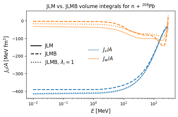
Note that, when we set \(\lambda_i=1\), neglecting the renormalization, JLM and JLMB nearly agree. The bulk of difference in the energy dependence of JLM and JLMB comes from the renormalization as opposed to the isovector effect or the ILDA. The notable exception to this is the imaginary part below \(\sim 200\) MeV where the Lane consistency uniformly decreases absorptive strength for neutrons on the neutron rich \(^{208}\)Pb.
Comparison of ways to compue the Coulomb potential from the proton density
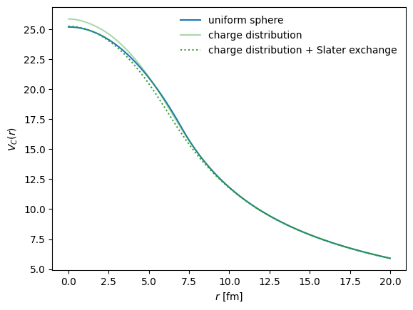
There are a few options built into jitr.folding.ILDAFolder. One can:
use the analytic, oft-used, uniform sphere convention, with the Coulomb radius determined friom a given proton density
use the full direct Coulomb potential
use the full Coulomb potential using the Slater local approximation to the exchange term
1rho_p_q = folder.interp_to_quad(R, rho_p_d1m)
2V_Coulomb_uniform_sphere = folder.V_coulomb(rho_p_q, mode="uniform_sphere")
3V_Coulomb_full = folder.V_coulomb(rho_p_q, mode="density")
4V_Coulomb_full_exchange = folder.V_coulomb(
5    rho_p_q, mode="density", include_exchange=True
6)
 1plt.plot(folder.r_q, V_Coulomb_uniform_sphere, label="uniform sphere")
 2plt.plot(
 3    folder.r_q,
 4    V_Coulomb_full,
 5    alpha=0.4,
 6    color="tab:green",
 7    label="charge distribution",
 8)
 9plt.plot(
10    folder.r_q,
11    V_Coulomb_full_exchange,
12    ":",
13    color="tab:green",
14    label="charge distribution + Slater exchange",
15)
16plt.legend(framealpha=0)
17plt.xlabel("$r$ [fm]")
18plt.ylabel("$V_C(r)$")
Text(0, 0.5, '$V_C(r)$')
Comparison of JLM and JLMB cross section predictions
Finally, we set up as Solver and compare cross sections predictions.
1from jitr import reactions, rmatrix, utils, xs
 1# calculate kinematics for a given lab energy
 2energy_lab = 60
 3projectile = proton
 4reaction = reactions.Reaction(target=target, projectile=proton, process="el")
 5kinematics = reaction.kinematics(energy_lab)
 6
 7# set the channel radius, number of nodes, and number of partial waves
 8interaction_range_fm = 1.2 * (target[0] ** (1 / 3)) + 2
 9channel_radius_dimensionless = utils.suggested_dimensionless_channel_radius(
10    interaction_range_fm, kinematics.k
11)
12channel_radius = channel_radius_dimensionless / kinematics.k
13N = utils.suggested_basis_size(channel_radius_dimensionless)
14lmax = 60
15
16# build a solver for the system and reaction of interest
17print(f"Compiling solver for {reaction} at {energy_lab} MeV")
18print(f" - channel radius {channel_radius:1.2f} fm")
19print(f" - {N} nodes")
20print(f" - {lmax} partial waves")
21
22solver = xs.elastic.DifferentialWorkspace.build_from_system(
23    reaction=reaction,
24    kinematics=kinematics,
25    channel_radius_fm=channel_radius,
26    solver=rmatrix.Solver(N),
27    lmax=lmax,
28    angles=np.linspace(0.1, np.pi, 180),
29)
30rgrid = solver.radial_grid()
31# jit warmup
32_ = solver.xs(central_potential=np.zeros_like(solver.radial_grid()))
33print("Done!")
Compiling solver for 208-Pb(p,el) at 60 MeV
 - channel radius 12.77 fm
 - 35 nodes
 - 60 partial waves
Done!
Now let’s compare the effects of the LDA vs. the ILDA on a differential cross section. We will use JLM and JLMB without the the energy renormalization (\(\lambda_i=1\)).
 1def get_potentials(solver, reaction, r_grid, rho_n, rho_p):
 2    rho_n_q = folder.interp_to_quad(r_grid, rho_n)
 3    rho_p_q = folder.interp_to_quad(r_grid, rho_p)
 4    V_C_q = folder.V_coulomb(
 5        rho_p_q,
 6        mode="density",
 7        include_exchange=True,
 8    )
 9    V_C = folder.V_coulomb(
10        rho_p_q,
11        mode="density",
12        include_exchange=True,
13        r_out=solver.radial_grid(),
14    )
15    jlmb_kwargs = {}
16    jlm_kwargs = {}
17    if reaction.projectile == proton:
18        jlmb_kwargs = {
19            "V_C": V_C_q,
20            "parameterization": "talys",
21        }
22        jlm_kwargs = {
23            "V_C": V_C,
24            "parameterization": "talys",
25        }
26    V_jlmb, W_jlmb = jlm.potential_JLMB(
27        folder,
28        rho_n_q,
29        rho_p_q,
30        reaction.projectile,
31        reaction.target,
32        kinematics.Ecm,
33        **jlmb_kwargs,
34        r_out=solver.radial_grid(),
35    )
36    V_jlm, W_jlm = jlm.potential_JLM(
37        solver.radial_grid(),
38        np.interp(solver.radial_grid(), r_grid, rho_n + rho_p),
39        reaction.projectile,
40        reaction.target,
41        kinematics.Ecm,
42        **jlm_kwargs,
43    )
44    return V_C, (V_jlm, W_jlm), (V_jlmb, W_jlmb)
1V_C, (V_jlm, W_jlm), (V_jlmb, W_jlmb) = get_potentials(
2    solver, reaction, R, rho_n_d1m, rho_p_d1m
3)
 1%%time
 2rho_n_q = folder.interp_to_quad(R, rho_n_d1m)
 3rho_p_q = folder.interp_to_quad(R, rho_p_d1m)
 4xs_jlm = solver.xs(
 5    central_potential=V_jlm + 1j * W_jlm,
 6    coulomb_potential=V_C,
 7)
 8xs_jlmb = solver.xs(
 9    central_potential=V_jlmb + 1j * W_jlmb,
10    coulomb_potential=V_C,
11)
CPU times: user 12.4 ms, sys: 968 μs, total: 13.4 ms
Wall time: 12.4 ms
1plt.plot(np.rad2deg(solver.angles), xs_jlm.dsdo / solver.rutherford, label="JLM")
2plt.plot(np.rad2deg(solver.angles), xs_jlmb.dsdo / solver.rutherford, label="JLMB")
3plt.xlabel(r"$\theta$ [deg]")
4plt.ylabel(r"$(d\sigma/d\Omega) / (d\sigma / d\Omega)_{R} $")
5plt.title(f"JLM vs. JLMB for ${reaction.reaction_latex}$ at {kinematics.Elab} MeV")
6plt.legend()
7plt.tight_layout()
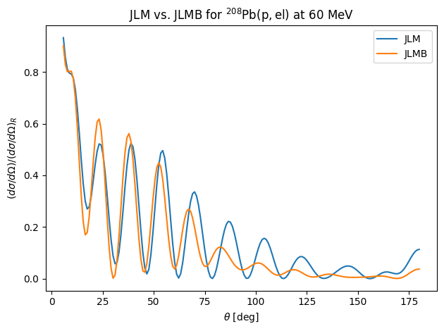
The ILDA produces more diffuse surfaces, so the diffraction oscillations become less pronounced.
Effect of densities on cross sections
 1# calculate kinematics for a given lab energy
 2energy_lab = 20
 3projectile = neutron
 4reaction = reactions.Reaction(target=target, projectile=projectile, process="el")
 5kinematics = reaction.kinematics(energy_lab)
 6
 7# set the channel radius, number of nodes, and number of partial waves
 8interaction_range_fm = 1.2 * (target[0] ** (1 / 3)) + 2
 9channel_radius_dimensionless = utils.suggested_dimensionless_channel_radius(
10    interaction_range_fm, kinematics.k
11)
12channel_radius = channel_radius_dimensionless / kinematics.k
13N = utils.suggested_basis_size(channel_radius_dimensionless)
14lmax = 60
15
16# build a solver for the system and reaction of interest
17print(f"Compiling solver for {reaction} at {energy_lab} MeV")
18print(f" - channel radius {channel_radius:1.2f} fm")
19print(f" - {N} nodes")
20print(f" - {lmax} partial waves")
21
22solver = xs.elastic.DifferentialWorkspace.build_from_system(
23    reaction=reaction,
24    kinematics=kinematics,
25    channel_radius_fm=channel_radius,
26    solver=rmatrix.Solver(N),
27    lmax=lmax,
28    angles=np.linspace(0.1, np.pi, 180),
29)
30rgrid = solver.radial_grid()
31# jit warmup
32_ = solver.xs(central_potential=np.zeros_like(solver.radial_grid()))
33print("Done!")
Compiling solver for 208-Pb(n,el) at 20 MeV
 - channel radius 15.50 fm
 - 25 nodes
 - 60 partial waves
Done!
 1%%time
 2densities = {
 3    label: (rho_n, rho_p)
 4    for label, rho_n, rho_p in [
 5        ("2pF", rho_n_2pf(R), rho_p_2pf(R)),
 6        ("bskg3", rho_n_bskg3, rho_p_bskg3),
 7        ("d1m", rho_n_d1m, rho_p_d1m),
 8    ]
 9}
10results_jlmb = {}
11results_jlm = {}
12
13for label, (rho_n, rho_p) in densities.items():
14    V_C, (V_jlm, W_jlm), (V_jlmb, W_jlmb) = get_potentials(
15        solver, reaction, R, rho_n, rho_p
16    )
17    results_jlm[label] = solver.xs(
18        central_potential=V_jlm + 1j * W_jlm,
19    )
20    results_jlmb[label] = solver.xs(
21        central_potential=V_jlmb + 1j * W_jlmb,
22    )
CPU times: user 24.7 ms, sys: 974 μs, total: 25.7 ms
Wall time: 23.9 ms
 1fig, ax = plt.subplots(1, 1, figsize=(6, 3))
 2for label in densities.keys():
 3    ax.plot(
 4        np.rad2deg(solver.angles),
 5        results_jlmb[label].dsdo,
 6        "--",
 7        alpha=0.7,
 8        color=colors[label],
 9        label=label,
10    )
11    # ax.plot(np.rad2deg(solver.angles), xs_jlmb.dsdo / solver.rutherford, color=colors[label], label=label)
12
13ax.set_xlabel(r"$\theta$ [deg]")
14ax.set_ylabel(r"$d\sigma/d\Omega$ [mb/Sr]")
15ax.set_yscale("log")
16plt.legend(ncol=3, framealpha=0)
17plt.tight_layout()
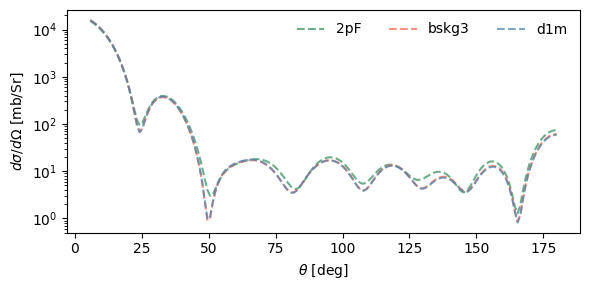
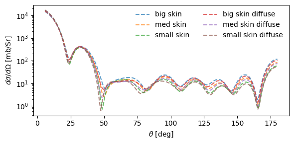
Let’s try tweaking some 2pF densities by hand, and seeing what effect it has.
 1goofy_densities = {
 2    "big skin": (
 3        TwoParameterFermiDensity(R=6.8, a=0.55, N=126)(R),
 4        TwoParameterFermiDensity(R=6.0, a=0.547, N=82)(R),
 5    ),
 6    "med skin": (
 7        TwoParameterFermiDensity(R=6.8, a=0.55, N=126)(R),
 8        TwoParameterFermiDensity(R=6.3, a=0.547, N=82)(R),
 9    ),
10    "small skin": (
11        TwoParameterFermiDensity(R=6.8, a=0.55, N=126)(R),
12        TwoParameterFermiDensity(R=6.6, a=0.547, N=82)(R),
13    ),
14    "big skin diffuse": (
15        TwoParameterFermiDensity(R=6.8, a=0.6, N=126)(R),
16        TwoParameterFermiDensity(R=6.0, a=0.6, N=82)(R),
17    ),
18    "med skin diffuse": (
19        TwoParameterFermiDensity(R=6.8, a=0.6, N=126)(R),
20        TwoParameterFermiDensity(R=6.3, a=0.6, N=82)(R),
21    ),
22    "small skin diffuse": (
23        TwoParameterFermiDensity(R=6.8, a=0.6, N=126)(R),
24        TwoParameterFermiDensity(R=6.6, a=0.6, N=82)(R),
25    ),
26}
 1%%time
 2results_jlmb = {}
 3results_jlm = {}
 4
 5for label, (rho_n, rho_p) in goofy_densities.items():
 6    V_C, (V_jlm, W_jlm), (V_jlmb, W_jlmb) = get_potentials(
 7        solver, reaction, R, rho_n, rho_p
 8    )
 9    results_jlm[label] = solver.xs(
10        central_potential=V_jlm + 1j * W_jlm,
11    )
12    results_jlmb[label] = solver.xs(
13        central_potential=V_jlmb + 1j * W_jlmb,
14    )
CPU times: user 48.7 ms, sys: 0 ns, total: 48.7 ms
Wall time: 48.9 ms
 1fig, ax = plt.subplots(1, 1, figsize=(6, 3))
 2for label in goofy_densities.keys():
 3    ax.plot(
 4        np.rad2deg(solver.angles),
 5        results_jlmb[label].dsdo,
 6        "--",
 7        alpha=0.7,
 8        label=label,
 9    )
10    # ax.plot(np.rad2deg(solver.angles), xs_jlmb.dsdo / solver.rutherford, color=colors[label], label=label)
11
12ax.set_xlabel(r"$\theta$ [deg]")
13ax.set_ylabel(r"$d\sigma/d\Omega$ [mb/Sr]")
14ax.set_yscale("log")
15plt.legend(ncol=2, framealpha=0)
16plt.tight_layout()