Channel-radius convergence study for elastic scattering
This notebook investigates how the chosen channel radius affects a realistic elastic-scattering calculation. It is most helpful once you are tuning solver settings and want a concrete convergence study to copy.
1import numpy as np
2from IPython.display import Math, display
3from periodictable import elements
1from matplotlib import pyplot as plt
1from tqdm import tqdm
2
3import jitr
Set up the system
1A, Z = (208, 82)
1name_core = str(elements[Z].symbol)
2display(Math(f"^{{{A}}} \\rm{{{name_core}}}"))
\[\displaystyle ^{208} \rm{Pb}\]
1neutron = (1, 0)
2proton = (1, 1)
3projectile = proton
4target = (A, Z)
Grab samples
1# we have 416 samples from the KDUQ posterior
2kduq_omp_samples = jitr.optical_potentials.kduq.get_samples(projectile)
Set up the solvers
1lab_energy_grid = np.array([30, 60])
1angles = np.linspace(0.01, np.pi, 120)
1channel_radii = np.arange(10, 35, 2)
2channel_radii
array([10, 12, 14, 16, 18, 20, 22, 24, 26, 28, 30, 32, 34])
1reaction = jitr.reactions.Reaction(target=target, projectile=projectile, process="EL")
 1def set_up_grid(core, lab_energy_grid):
 2    solvers = []
 3    for _i, Elab in enumerate(lab_energy_grid):
 4        kinematics = reaction.kinematics(Elab)
 5        solvers.append([])
 6        for channel_radius in channel_radii:
 7            N = jitr.utils.suggested_basis_size(channel_radius * kinematics.k)
 8            lmax = int(max(30, kinematics.k * channel_radius))
 9            print(
10                f"E={Elab:1.1f} MeV, ",
11                f"R={channel_radius:1.1f} fm, ",
12                f"{kinematics.k * channel_radius / (2 * np.pi):1.1f} λ's, ",
13                f"nodes: {N}, ",
14                f"max l: {lmax}",
15            )
16            solvers[-1].append(
17                jitr.xs.elastic.DifferentialWorkspace.build_from_system(
18                    reaction=reaction,
19                    kinematics=kinematics,
20                    angles=angles,
21                    channel_radius_fm=channel_radius,
22                    solver=jitr.rmatrix.Solver(N),
23                    lmax=lmax,
24                    smatrix_abs_tol=1e-6,
25                )
26            )
27    return solvers
1solvers = set_up_grid(target, lab_energy_grid)
E=30.0 MeV,  R=10.0 fm,  1.9 λ's,  nodes: 20,  max l: 30
E=30.0 MeV,  R=12.0 fm,  2.3 λ's,  nodes: 25,  max l: 30
E=30.0 MeV,  R=14.0 fm,  2.7 λ's,  nodes: 30,  max l: 30
E=30.0 MeV,  R=16.0 fm,  3.1 λ's,  nodes: 35,  max l: 30
E=30.0 MeV,  R=18.0 fm,  3.5 λ's,  nodes: 35,  max l: 30
E=30.0 MeV,  R=20.0 fm,  3.8 λ's,  nodes: 40,  max l: 30
E=30.0 MeV,  R=22.0 fm,  4.2 λ's,  nodes: 45,  max l: 30
E=30.0 MeV,  R=24.0 fm,  4.6 λ's,  nodes: 50,  max l: 30
E=30.0 MeV,  R=26.0 fm,  5.0 λ's,  nodes: 50,  max l: 31
E=30.0 MeV,  R=28.0 fm,  5.4 λ's,  nodes: 55,  max l: 33
E=30.0 MeV,  R=30.0 fm,  5.8 λ's,  nodes: 60,  max l: 36
E=30.0 MeV,  R=32.0 fm,  6.1 λ's,  nodes: 65,  max l: 38
E=30.0 MeV,  R=34.0 fm,  6.5 λ's,  nodes: 70,  max l: 41
E=60.0 MeV,  R=10.0 fm,  2.7 λ's,  nodes: 30,  max l: 30
E=60.0 MeV,  R=12.0 fm,  3.3 λ's,  nodes: 35,  max l: 30
E=60.0 MeV,  R=14.0 fm,  3.8 λ's,  nodes: 40,  max l: 30
E=60.0 MeV,  R=16.0 fm,  4.4 λ's,  nodes: 45,  max l: 30
E=60.0 MeV,  R=18.0 fm,  4.9 λ's,  nodes: 50,  max l: 30
E=60.0 MeV,  R=20.0 fm,  5.5 λ's,  nodes: 55,  max l: 34
E=60.0 MeV,  R=22.0 fm,  6.0 λ's,  nodes: 65,  max l: 37
E=60.0 MeV,  R=24.0 fm,  6.6 λ's,  nodes: 70,  max l: 41
E=60.0 MeV,  R=26.0 fm,  7.1 λ's,  nodes: 75,  max l: 44
E=60.0 MeV,  R=28.0 fm,  7.7 λ's,  nodes: 80,  max l: 48
E=60.0 MeV,  R=30.0 fm,  8.2 λ's,  nodes: 85,  max l: 51
E=60.0 MeV,  R=32.0 fm,  8.8 λ's,  nodes: 90,  max l: 54
E=60.0 MeV,  R=34.0 fm,  9.3 λ's,  nodes: 95,  max l: 58
Run the calculations
1N = 100  # number of samples to draw from each posterior
2draws_kduq = np.random.choice(len(kduq_omp_samples), size=N)
 1xs = np.zeros((N, lab_energy_grid.size, channel_radii.size, angles.size))
 2for i, sample in enumerate(tqdm(kduq_omp_samples[draws_kduq, :])):
 3    for j, _Ecm in enumerate(lab_energy_grid):
 4        for k, _channel_radius in enumerate(channel_radii):
 5            solver = solvers[j][k]
 6            rgrid = solver.radial_grid()
 7            central_params, spin_orbit_params, coulomb_params = (
 8                jitr.optical_potentials.kduq.calculate_params(
 9                    projectile,
10                    target,
11                    solver.kinematics.Elab,
12                    *sample,
13                )
14            )
15            x = solver.xs(
16                jitr.optical_potentials.kduq.central(rgrid, *central_params),
17                jitr.optical_potentials.kduq.spin_orbit(rgrid, *spin_orbit_params),
18                jitr.optical_potentials.kduq.coulomb_charged_sphere(
19                    rgrid, *coulomb_params
20                ),
21            )
22            if projectile == proton:
23                x.dsdo /= solver.rutherford
24            xs[i, j, k, :] = x.dsdo
100%|███████████████████████████████████████████████████████████████████████████████| 100/100 [01:34<00:00, 1.06it/s]
1benchmark = xs[:, :, -1:, :]
2tests = xs[:, :, :-1, :]
3
4diff = np.median(tests - benchmark, axis=0)
5rel_diff = np.median((tests - benchmark) / benchmark, axis=0)
6log_abs_diff = np.median(np.log(np.abs(tests - benchmark)), axis=0)
7xs_median = np.median(xs, axis=0)
Visualize the results
1import matplotlib.cm as cm
2import matplotlib.colors as mcolors
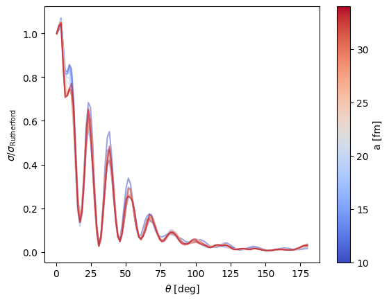
1Eidx = 1
2print(f"Plots for E = {lab_energy_grid[Eidx]} MeV")
Plots for E = 60 MeV
 1cmap = plt.get_cmap("coolwarm")
 2norm = mcolors.Normalize(vmin=min(channel_radii), vmax=max(channel_radii))
 3sm = cm.ScalarMappable(norm=norm, cmap=cmap)
 4sm.set_array([])
 5
 6for i in range(len(channel_radii)):
 7    a = channel_radii[i]
 8    color = sm.to_rgba(a)
 9    plt.plot(angles * 180 / np.pi, xs_median[Eidx, i, :], color=color, alpha=0.5)
10plt.gcf().colorbar(sm, ax=plt.gca(), label="a [fm]")
11plt.xlabel(r"$\theta$ [deg]")
12
13
14if projectile == neutron:
15    plt.yscale("log")
16    plt.ylabel(r"$\frac{d\sigma}{d\Omega}$ [mb/Sr]")
17else:
18    plt.ylabel(r"$\sigma / \sigma_{\text{Rutherford}}$")
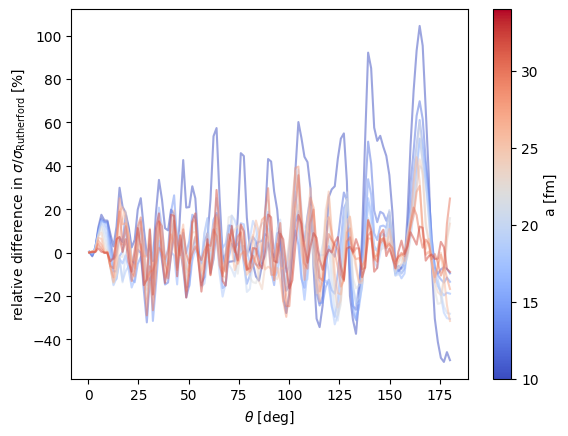
 1for i in range(len(channel_radii) - 1):
 2    a = channel_radii[i]
 3    color = sm.to_rgba(a)
 4    plt.plot(angles * 180 / np.pi, rel_diff[Eidx, i, :] * 100, color=color, alpha=0.5)
 5plt.gcf().colorbar(sm, ax=plt.gca(), label="a [fm]")
 6plt.xlabel(r"$\theta$ [deg]")
 7if projectile == neutron:
 8    plt.ylabel(r"relative difference in $\frac{d\sigma}{d\Omega}$ [%]")
 9else:
10    plt.ylabel(r"relative difference in $\sigma / \sigma_{\text{Rutherford}}$ [%]")
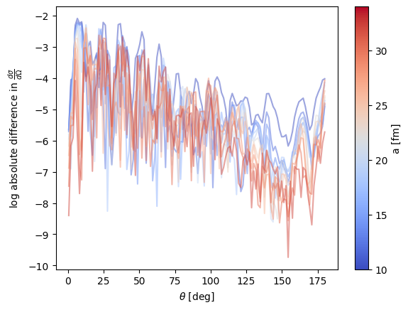
1for i in range(len(channel_radii) - 1):
2    a = channel_radii[i]
3    color = sm.to_rgba(a)
4    plt.plot(angles * 180 / np.pi, log_abs_diff[Eidx, i, :], color=color, alpha=0.5)
5plt.gcf().colorbar(sm, ax=plt.gca(), label="a [fm]")
6plt.xlabel(r"$\theta$ [deg]")
7plt.ylabel(r"log absolute difference in $\frac{d\sigma}{d\Omega}$")
Text(0, 0.5, 'log absolute difference in $\\frac{d\\sigma}{d\\Omega}$')
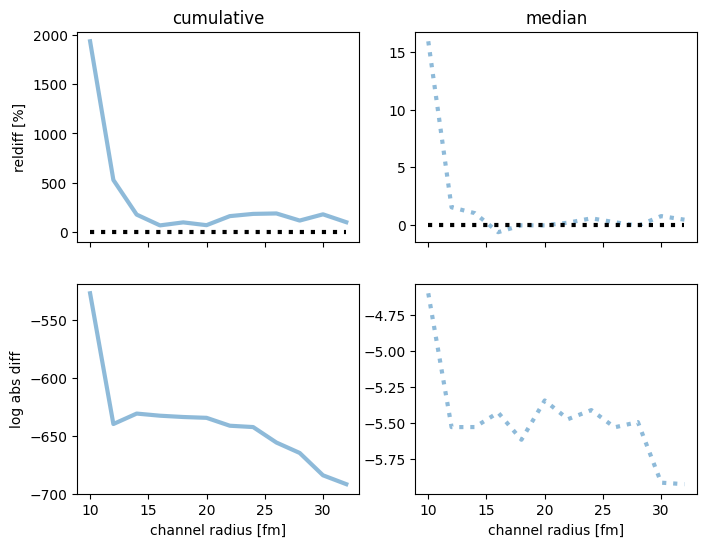
 1cum_diff = np.sum(diff[Eidx, ...], axis=-1)
 2cum_rel_diff = np.sum(rel_diff[Eidx, ...] * 100, axis=-1)
 3cum_log_abs_diff = np.sum(log_abs_diff[Eidx, ...], axis=-1)
 4med_diff = np.median(diff[Eidx, ...], axis=-1)
 5med_rel_diff = np.median(rel_diff[Eidx, ...] * 100, axis=-1)
 6med_log_abs_diff = np.median(log_abs_diff[Eidx, ...], axis=-1)
 7
 8fig, axes = plt.subplots(2, 2, sharex=True, figsize=(8, 6))
 9axes[0, 0].plot(
10    channel_radii[:-1],
11    cum_rel_diff,
12    alpha=0.5,
13    linewidth=3,
14)
15axes[0, 1].plot(
16    channel_radii[:-1],
17    med_rel_diff,
18    ":",
19    alpha=0.5,
20    linewidth=3,
21)
22axes[0, 0].plot(
23    channel_radii[:-1],
24    np.zeros_like(channel_radii[:-1]),
25    "k:",
26    linewidth=3,
27)
28axes[0, 1].plot(
29    channel_radii[:-1],
30    np.zeros_like(channel_radii[:-1]),
31    "k:",
32    linewidth=3,
33)
34axes[1, 0].plot(
35    channel_radii[:-1],
36    cum_log_abs_diff,
37    alpha=0.5,
38    linewidth=3,
39)
40axes[1, 1].plot(
41    channel_radii[:-1],
42    med_log_abs_diff,
43    ":",
44    alpha=0.5,
45    linewidth=3,
46)
47axes[-1, 0].set_xlabel("channel radius [fm]")
48axes[-1, 1].set_xlabel("channel radius [fm]")
49axes[0, 0].set_title("cumulative")
50axes[0, 1].set_title("median")
51
52axes[0, 0].set_ylabel("reldiff [%]")
53axes[1, 0].set_ylabel("log abs diff")
Text(0, 0.5, 'log abs diff')