Differential cross-section uncertainty propagation with KDUQ
KDUQ is an uncertainty-quantified global optical potential. This notebook shows how to sample that posterior information, run the solver repeatedly, and summarize the resulting uncertainty in differential cross sections.
1# import stuff for nice plotting
2import matplotlib.pyplot as plt
3import numpy as np
4from tqdm import tqdm
5
6import jitr
1from jitr.optical_potentials import kduq
 1#  elastic reaction
 2target = (54, 26)
 3proton = (1, 1)
 4neutron = (1, 0)
 5projectile = proton
 6
 7reaction = jitr.reactions.ElasticReaction(
 8    target=target,
 9    projectile=projectile,
10)
11
12# energy
13Elab = 35
14kinematics = reaction.kinematics(Elab)
15
16# for plotting differential xs
17angles = np.linspace(0.1, np.pi, 180)
18
19# Lagrange Mesh
20core_solver = jitr.rmatrix.Solver(40)
Set up the solver for differential cross sections
 1# get kinematics and parameters for this experiment
 2
 3a = jitr.utils.interaction_range(target[0]) * kinematics.k + np.pi * 2
 4N = jitr.utils.suggested_basis_size(a)
 5assert N < core_solver.kernel.quadrature.nbasis
 6channel_radius_fm = a / kinematics.k
 7
 8# build solver
 9solver = jitr.xs.elastic.DifferentialWorkspace.build_from_system(
10    reaction=reaction,
11    kinematics=kinematics,
12    channel_radius_fm=channel_radius_fm,
13    solver=core_solver,
14    lmax=50,
15    angles=angles,
16)
Sample the KDUQ posterior
1help(kduq.get_samples)
Help on function get_samples in module jitr.optical_potentials.kduq:

get_samples(projectile: tuple[int, int], posterior: str = 'federal') -> numpy.ndarray
    Get the posterior samples for the given projectile (neutron or
    proton) from the KDUQ Federal or Democratic posteriors.

    See [Pruitt, et al., 2023]
    (https://journals.aps.org/prc/pdf/10.1103/PhysRevC.107.014602) for
    details on the KDUQ posteriors.

    :param projectile: tuple A tuple representing the projectile, with format (Ap,
                       Zp), where Ap is the mass number and Zp is the atomic number.
                       Must be either (1, 0) for neutron or (1, 1) for proton.
    :param posterior: str Which KDUQ posterior to return samples from. Must be
                      either "federal" or "democratic". Defaults to "federal".
    :returns: An array of shape (NUM_POSTERIOR_SAMPLES, num_params) containing the
              posterior samples for the given projectile, where num_params is the
              number of parameters in the Koning-Delaroche potential, and the
              parameters are ordered according to the order set by the
              get_param_names function.
    :rtype: np.ndarray
1kduq_samples = kduq.get_samples(projectile)
Set up the potential
Let’s take a look at the functionality built into jitr:
1omp = kduq.KDUQ(projectile)
2help(omp)
Help on KDUQ in module jitr.optical_potentials.kduq object:

class KDUQ(jitr.optical_potentials.omp.SingleChannelOpticalModel)
 |  KDUQ(projectile: tuple)
 |
 |  Koning-Delaroche Uncertainty Quantification (KDUQ) optical
 |  potential model.
 |
 |  Method resolution order:
 |      KDUQ
 |      jitr.optical_potentials.omp.SingleChannelOpticalModel
 |      builtins.object
 |
 |  Methods defined here:
 |
 |  __init__(self, projectile: tuple)
 |      Initialize self.  See help(type(self)) for accurate signature.
 |
 |  evaluate(self, rgrid: float | numpy.ndarray, reaction: jitr.reactions.reaction.Reaction, kinematics: jitr.utils.kinematics.ChannelKinematics, *params: float) -> tuple[complex | numpy.ndarray[tuple[typing.Any, ...], numpy.dtype[numpy.complex128]], complex | numpy.ndarray[tuple[typing.Any, ...], numpy.dtype[numpy.complex128]], float | numpy.ndarray[tuple[typing.Any, ...], numpy.dtype[numpy.float64]]]
 |      Evaluate the KDUQ central, spin-orbit, and Coulomb terms.
 |
 |  ----------------------------------------------------------------------
 |  Methods inherited from jitr.optical_potentials.omp.SingleChannelOpticalModel:
 |
 |  __call__(self, rgrid: 'ArrayOrScalar', reaction: 'reaction.Reaction', kinematics: 'kinematics.ChannelKinematics', *params: 'float') -> 'tuple[PotentialArray, PotentialArray, PotentialArray | ArrayOrScalar]'
 |      Call self as a function.
 |
 |  ----------------------------------------------------------------------
 |  Data descriptors inherited from jitr.optical_potentials.omp.SingleChannelOpticalModel:
 |
 |  __dict__
 |      dictionary for instance variables
 |
 |  __weakref__
 |      list of weak references to the object
1help(jitr.optical_potentials.kduq.central)
Help on function central in module jitr.optical_potentials.kduq:

central(r: float | numpy.ndarray, Vv: float, Rv: float, av: float, Wv: float, Rwv: float, awv: float, Wd: float, Rd: float, ad: float) -> complex | numpy.ndarray[tuple[typing.Any, ...], numpy.dtype[numpy.complex128]]
    Koning-Delaroche central terms at a given energy.

    This matches Eq. (7) in Koning and Delaroche (2003).

    :param r: float or np.ndarray The radius at which to evaluate the potential.
    :param Vv: float The real central depth.
    :param Rv: float The real central radius parameter.
    :param av: float The real central diffuseness parameter.
    :param Wv: float The imaginary volume depth.
    :param Rwv: float The imaginary volume radius parameter.
    :param awv: float The imaginary volume diffuseness parameter.
    :param Wd: float The imaginary surface depth.
    :param Rd: float The imaginary surface radius parameter.
    :param ad: float The imaginary surface diffuseness parameter.
1help(jitr.optical_potentials.kduq.spin_orbit)
Help on function spin_orbit in module jitr.optical_potentials.kduq:

spin_orbit(r: float | numpy.ndarray, Vso: float, Rso: float, aso: float, Wso: float, Rwso: float, awso: float) -> complex | numpy.ndarray[tuple[typing.Any, ...], numpy.dtype[numpy.complex128]]
    Koning-Delaroche spin-orbit terms at a given energy.

    This matches Eq. (7) in Koning and Delaroche (2003).

    :param r: float or np.ndarray The radius at which to evaluate the potential.
    :param Vso: float The real spin-orbit depth.
    :param Rso: float The real spin-orbit radius parameter.
    :param aso: float The real spin-orbit diffuseness parameter.
    :param Wso: float The imaginary spin-orbit depth.
    :param Rwso: float The imaginary spin-orbit radius parameter.
    :param awso: float The imaginary spin-orbit diffuseness parameter.
1help(jitr.optical_potentials.potential_forms.coulomb_charged_sphere)
Help on function coulomb_charged_sphere in module jitr.optical_potentials.potential_forms:

coulomb_charged_sphere(r: 'ArrayOrScalar', zz: 'float', r_c: 'float') -> 'ArrayOrScalar'
    Return the Coulomb potential of a uniformly charged sphere.
Run the calculation
This should demonstrate how the KDUQ class (omp) is built to interface with solver, which is an instance of jitr.xs.elastic.DifferentialWorkspace. This is how calculations are done in jitr.
1kduq_xs = np.zeros((len(angles), kduq.NUM_POSTERIOR_SAMPLES))
2rgrid = solver.radial_grid()
3
4for j, sample in enumerate(tqdm(kduq_samples)):
5    central_term, spin_orbit_term, coulomb_term = omp(
6        rgrid, reaction, kinematics, *sample
7    )
8    xs = solver.xs(central_term, spin_orbit_term, coulomb_term)
9    kduq_xs[:, j] = xs.dsdo / solver.rutherford
 95%|██████████████████████████████████████████████████████████████████████████▍   | 397/416 [00:11<00:00, 229.31it/s]/home/kyle/umich/jitr/src/jitr/optical_potentials/kduq.py:467: RuntimeWarning: overflow encountered in exp
  d2 = d2_0 + d2_A / (1 + np.exp((A - d2_A3) / d2_A2))
100%|███████████████████████████████████████████████████████████████████████████████| 416/416 [00:11<00:00, 36.63it/s]
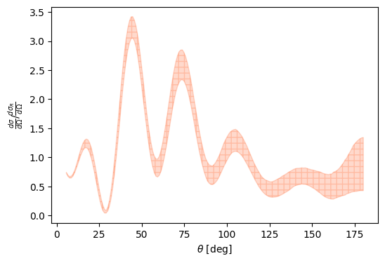
Compute intervals and plot results
1kduq_pred_post = np.percentile(kduq_xs, [16, 84], axis=1)
 1fig, ax = plt.subplots(1, 1, figsize=(6, 4))
 2ax.fill_between(
 3    angles * 180 / np.pi,
 4    kduq_pred_post[0],  # / solver.rutherford,
 5    kduq_pred_post[1],  # / solver.rutherford,
 6    color="#ff4500",
 7    hatch="|-|-",
 8    alpha=0.2,
 9)
10plt.xlabel(r"$\theta$ [deg]")
11plt.ylabel(r"$\frac{d \sigma}{d\Omega} / \frac{d \sigma_{R}}{d\Omega} $")
Text(0, 0.5, '$\\frac{d \\sigma}{d\\Omega} / \\frac{d \\sigma_{R}}{d\\Omega} $')
1# NBVAL_CHECK_OUTPUT
2print(f"{kduq_pred_post[1][9]:1.6f}")
1.163423
In fact, KDUQ is just one definition of a global optical potential. jitr also has others built in:
1help(jitr.optical_potentials.wlh.WLH)
Help on class WLH in module jitr.optical_potentials.wlh:

class WLH(jitr.optical_potentials.omp.SingleChannelOpticalModel)
 |  WLH(projectile: tuple)
 |
 |  The Whitehead-Lim-Holt global optical potential for nucleon-nucleus
 |  scattering.
 |
 |  Method resolution order:
 |      WLH
 |      jitr.optical_potentials.omp.SingleChannelOpticalModel
 |      builtins.object
 |
 |  Methods defined here:
 |
 |  __init__(self, projectile: tuple)
 |      Initialize self.  See help(type(self)) for accurate signature.
 |
 |  evaluate(self, rgrid: float | numpy.ndarray[tuple[typing.Any, ...], numpy.dtype[numpy.float64]], reaction: jitr.reactions.reaction.Reaction, kinematics: jitr.utils.kinematics.ChannelKinematics, *params: float) -> tuple[complex | numpy.ndarray[tuple[typing.Any, ...], numpy.dtype[numpy.complex128]], complex | numpy.ndarray[tuple[typing.Any, ...], numpy.dtype[numpy.complex128]], float | numpy.ndarray[tuple[typing.Any, ...], numpy.dtype[numpy.float64]]]
 |      Evaluate the central, spin-orbit, and Coulomb terms of the WLH
 |      potential on the given radial grid for the specified reaction and
 |      kinematics, using the provided potential parameters.
 |
 |
 |      :param reaction: Reaction The reaction for which to calculate the
 |                       parameters.
 |      :param kinematics: ChannelKinematics The kinematics of the reaction
 |                         channel.s
 |      :param uv0, uv1, ..., aso1: float Parameters of the WLH potential. See
 |                                  [Whitehead et al., 2021]
 |                                  (https://journals.aps.org/prl/abstract/10.1103/PhysRevLett.127.182502)
 |                                  for details.
 |      :returns: U_central: np.ndarray Central term of the optical potential
 |                evaluated on the radial grid; U_spin_orbit: np.ndarray
 |                Spin-orbit term of the optical potential evaluated on the
 |                radial grid; U_coulomb: np.ndarray Coulomb term of the optical
 |                potential evaluated on the radial grid
 |      :rtype: tuple[U_central, U_spin_orbit, U_coulomb]
 |
 |  ----------------------------------------------------------------------
 |  Methods inherited from jitr.optical_potentials.omp.SingleChannelOpticalModel:
 |
 |  __call__(self, rgrid: 'ArrayOrScalar', reaction: 'reaction.Reaction', kinematics: 'kinematics.ChannelKinematics', *params: 'float') -> 'tuple[PotentialArray, PotentialArray, PotentialArray | ArrayOrScalar]'
 |      Call self as a function.
 |
 |  ----------------------------------------------------------------------
 |  Data descriptors inherited from jitr.optical_potentials.omp.SingleChannelOpticalModel:
 |
 |  __dict__
 |      dictionary for instance variables
 |
 |  __weakref__
 |      list of weak references to the object
1help(jitr.optical_potentials.chuq.CHUQ)
Help on class CHUQ in module jitr.optical_potentials.chuq:

class CHUQ(jitr.optical_potentials.omp.SingleChannelOpticalModel)
 |  Chapel-Hill Uncertainty Quantification (CHUQ) optical
 |  potential model.
 |
 |  Note that CH89 is Lane consistent, so the same parameters can be
 |  used for both neutron and proton projectiles.
 |
 |  Method resolution order:
 |      CHUQ
 |      jitr.optical_potentials.omp.SingleChannelOpticalModel
 |      builtins.object
 |
 |  Methods defined here:
 |
 |  __init__(self)
 |      Initialize self.  See help(type(self)) for accurate signature.
 |
 |  evaluate(self, rgrid: float | numpy.ndarray, reaction: jitr.reactions.reaction.Reaction, kinematics: jitr.utils.kinematics.ChannelKinematics, *params: float) -> tuple[complex | numpy.ndarray[tuple[typing.Any, ...], numpy.dtype[numpy.complex128]], complex | numpy.ndarray[tuple[typing.Any, ...], numpy.dtype[numpy.complex128]], float | numpy.ndarray[tuple[typing.Any, ...], numpy.dtype[numpy.float64]]]
 |      Evaluate the CHUQ central, spin-orbit, and Coulomb terms.
 |
 |  ----------------------------------------------------------------------
 |  Methods inherited from jitr.optical_potentials.omp.SingleChannelOpticalModel:
 |
 |  __call__(self, rgrid: 'ArrayOrScalar', reaction: 'reaction.Reaction', kinematics: 'kinematics.ChannelKinematics', *params: 'float') -> 'tuple[PotentialArray, PotentialArray, PotentialArray | ArrayOrScalar]'
 |      Call self as a function.
 |
 |  ----------------------------------------------------------------------
 |  Data descriptors inherited from jitr.optical_potentials.omp.SingleChannelOpticalModel:
 |
 |  __dict__
 |      dictionary for instance variables
 |
 |  __weakref__
 |      list of weak references to the object
In fact, these are all derived from jitr.optical_potentials.SingleChannelOpticalModel, which sets the interface between the model for the effective interaction and the solver. You can come up with your own optical model and derive your own class from jitr.optical_potentials.SingleChannelOpticalModel to plug it into jitr!
1help(jitr.optical_potentials.SingleChannelOpticalModel)
Help on class SingleChannelOpticalModel in module jitr.optical_potentials.omp:

class SingleChannelOpticalModel(builtins.object)
 |  SingleChannelOpticalModel(params: 'list[str]') -> 'None'
 |
 |  Base class for local single-channel optical potentials.
 |
 |  Methods defined here:
 |
 |  __call__(self, rgrid: 'ArrayOrScalar', reaction: 'reaction.Reaction', kinematics: 'kinematics.ChannelKinematics', *params: 'float') -> 'tuple[PotentialArray, PotentialArray, PotentialArray | ArrayOrScalar]'
 |      Call self as a function.
 |
 |  __init__(self, params: 'list[str]') -> 'None'
 |      Initialize self.  See help(type(self)) for accurate signature.
 |
 |  evaluate(self, rgrid: 'ArrayOrScalar', reaction: 'reaction.Reaction', kinematics: 'kinematics.ChannelKinematics', *params: 'float') -> 'tuple[PotentialArray, PotentialArray, PotentialArray | ArrayOrScalar]'
 |      Evaluate central, spin-orbit, and Coulomb terms on ``rgrid``.
 |
 |  ----------------------------------------------------------------------
 |  Data descriptors defined here:
 |
 |  __dict__
 |      dictionary for instance variables
 |
 |  __weakref__
 |      list of weak references to the object