Compare built-in uncertainty-quantified optical potentials
This notebook compares several uncertainty-quantified optical potentials on the same elastic-scattering observable.
1import matplotlib.pyplot as plt
2import numpy as np
3from tqdm import tqdm
4
5import jitr
1from jitr.optical_potentials import chuq, kduq, wlh
1#  elastic reaction
2target = (54, 26)
3proton = (1, 1)
4neutron = (1, 0)
5projectile = proton
6
7# for plotting differential xs
8angles = np.linspace(0.1, np.pi, 100)
1quantity = "dXS/dRuth"
2# quantity = "dXS/dA"
3assert not (projectile == neutron and quantity == "dXS/dRuth")
Retrieve comparison data
Let’s grab some data from EXFOR.
1#! pip install exfor-tools
2import exfor_tools
Using database version X4-2024-12-31 located in: /home/kyle/db/exfor/unpack_exfor-2024/X4-2024-12-31
1all_entries, failed_parses = exfor_tools.curate.query_for_entries(
2    exfor_tools.reaction.Reaction(target=target, projectile=projectile, process="El"),
3    quantity=quantity,
4    Einc_range=[7, 60],  # MeV
5)
6all_measurements = exfor_tools.curate.categorize_measurements_by_energy(all_entries)
1all_entries.keys()
dict_keys(['O0240', 'O0788', 'O1243'])
1all_entries_Ay, failed_parses = exfor_tools.curate.query_for_entries(
2    exfor_tools.reaction.Reaction(target=target, projectile=projectile, process="EL"),
3    quantity="Ay",
4    Einc_range=[7, 60],  # MeV
5)
6all_measurements_Ay = exfor_tools.curate.categorize_measurements_by_energy(
7    all_entries_Ay
8)
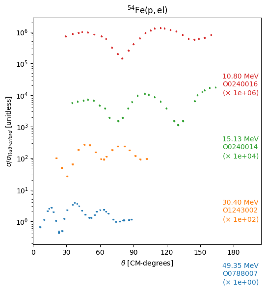
 1fig, ax = plt.subplots(1, 1, figsize=(6, 6))
 2exfor_keys = list(all_entries.keys())
 3exfor_tools.distribution.AngularDistribution.plot(
 4    all_measurements,
 5    ax,
 6    offsets=100,
 7    data_symbol=list(all_entries.values())[0].data_symbol,
 8    rxn_label=f"${list(all_entries.values())[0].reaction.reaction_latex}$",
 9    label_kwargs={
10        "label_offset_factor": 0.01,
11        "label_offset": True,
12        "label_exfor": True,
13        "label_xloc_deg": 170,
14        "label_energy_err": False,
15    },
16)
17ax.set_xlim([0, 205])
(0.0, 205.0)
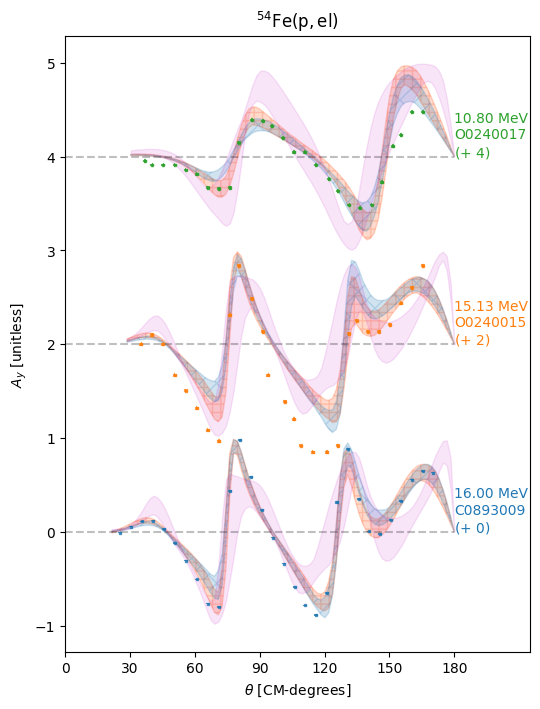
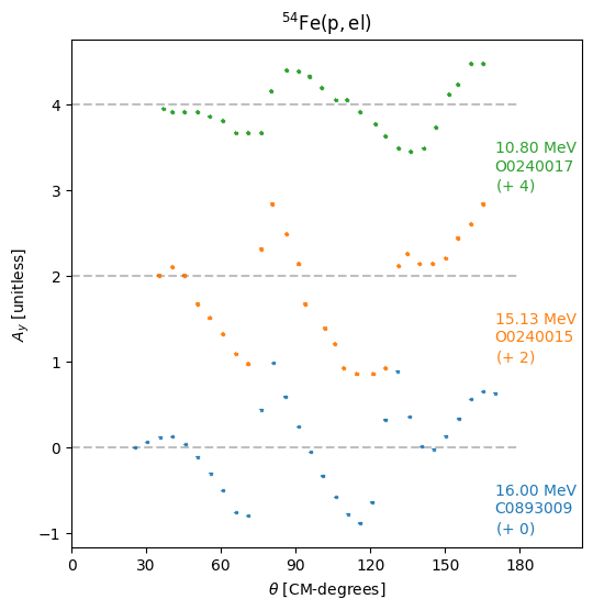
 1fig, ax = plt.subplots(1, 1, figsize=(6, 6))
 2exfor_keys = list(all_entries_Ay.keys())
 3exfor_tools.distribution.AngularDistribution.plot(
 4    all_measurements_Ay,
 5    ax,
 6    offsets=2,
 7    data_symbol=list(all_entries_Ay.values())[0].data_symbol,
 8    rxn_label=f"${list(all_entries.values())[0].reaction.reaction_latex}$",
 9    draw_baseline=True,
10    baseline_offset=0,
11    log=False,
12    label_kwargs={
13        "label_offset_factor": -1,
14        "label_offset": True,
15        "label_exfor": True,
16        "label_xloc_deg": 170,
17        "label_energy_err": False,
18    },
19)
20ax.set_xlim([0, 205])
(0.0, 205.0)
Set up the solver for differential cross sections
 1solvers = []
 2solvers_Ay = []
 3
 4reaction = jitr.reactions.ElasticReaction(
 5    target=target,
 6    projectile=projectile,
 7)
 8
 9
10for measurements in tqdm(all_measurements):
11    measurement = measurements[0]
12    Elab = measurement.Einc
13
14    # get kinematics and parameters for this experiment
15    kinematics = reaction.kinematics(Elab)
16
17    a = jitr.utils.interaction_range(target[0]) * kinematics.k + np.pi * 3
18    N = jitr.utils.suggested_basis_size(a)
19    channel_radius_fm = a / kinematics.k
20
21    solvers.append(
22        jitr.xs.elastic.DifferentialWorkspace.build_from_system(
23            reaction=reaction,
24            kinematics=kinematics,
25            channel_radius_fm=channel_radius_fm,
26            solver=jitr.rmatrix.Solver(N),
27            lmax=50,
28            angles=angles,
29        )
30    )
31
32for measurements in tqdm(all_measurements_Ay):
33    measurement = measurements[0]
34    Elab = measurement.Einc
35
36    # get kinematics and parameters for this experiment
37    kinematics = reaction.kinematics(Elab)
38
39    a = jitr.utils.interaction_range(target[0]) * kinematics.k + np.pi * 3
40    N = jitr.utils.suggested_basis_size(a)
41    channel_radius_fm = a / kinematics.k
42
43    solvers_Ay.append(
44        jitr.xs.elastic.DifferentialWorkspace.build_from_system(
45            reaction=reaction,
46            kinematics=kinematics,
47            channel_radius_fm=channel_radius_fm,
48            solver=jitr.rmatrix.Solver(N),
49            lmax=50,
50            angles=angles,
51        )
52    )
100%|███████████████████████████████████████████████████████████████████████████████████| 4/4 [00:29<00:00,  7.41s/it]
100%|███████████████████████████████████████████████████████████████████████████████████| 3/3 [00:41<00:00, 13.93s/it]
Run the uncertainty propagation
Sample posterior draws from each optical potential
1kduq_samples = kduq.get_samples(projectile)
2chuq_samples = chuq.get_samples()  # Lane consistent so no need to specify projectile
3wlh_samples = wlh.get_samples(projectile)
1kduq_omp = kduq.KDUQ(projectile)
2chuq_omp = chuq.CHUQ()
3wlh_omp = wlh.WLH(projectile)
 1def run_uq(omp, samples):
 2    xs_bands = []
 3    Ay_bands = []
 4
 5    for i in range(len(all_measurements)):
 6        xs_samples = np.zeros((len(angles), len(samples)))
 7        rgrid = solvers[i].radial_grid()
 8
 9        for j, sample in enumerate(tqdm(samples)):
10            central_term, spin_orbit_term, coulomb_term = omp(
11                rgrid, solvers[i].reaction, solvers[i].kinematics, *sample
12            )
13            xs = solvers[i].xs(central_term, spin_orbit_term, coulomb_term)
14            xs_samples[:, j] = xs.dsdo
15
16        xs_bands.append(np.percentile(xs_samples, [16, 84], axis=1))
17
18    for i in range(len(all_measurements_Ay)):
19        ay_samples = np.zeros((len(angles), len(samples)))
20        rgrid = solvers_Ay[i].radial_grid()
21
22        for j, sample in enumerate(tqdm(samples)):
23            central_term, spin_orbit_term, coulomb_term = omp(
24                rgrid, solvers_Ay[i].reaction, solvers_Ay[i].kinematics, *sample
25            )
26            xs = solvers_Ay[i].xs(central_term, spin_orbit_term, coulomb_term)
27            ay_samples[:, j] = xs.Ay
28
29        Ay_bands.append(np.percentile(ay_samples, [16, 84], axis=1))
30    return xs_bands, Ay_bands
KDUQ:
1kduq_pred_post, kduq_pred_post_Ay = run_uq(kduq_omp, kduq_samples)
 96%|██████████████████████████████████████████████████████████████████████████▋   | 398/416 [00:33<00:00, 119.19it/s]/home/kyle/umich/jitr/src/jitr/optical_potentials/kduq.py:467: RuntimeWarning: overflow encountered in exp
  d2 = d2_0 + d2_A / (1 + np.exp((A - d2_A3) / d2_A2))
100%|███████████████████████████████████████████████████████████████████████████████| 416/416 [00:34<00:00, 12.19it/s]
100%|██████████████████████████████████████████████████████████████████████████████| 416/416 [00:03<00:00, 110.59it/s]
100%|██████████████████████████████████████████████████████████████████████████████| 416/416 [00:02<00:00, 139.61it/s]
100%|██████████████████████████████████████████████████████████████████████████████| 416/416 [00:03<00:00, 131.76it/s]
100%|██████████████████████████████████████████████████████████████████████████████| 416/416 [00:02<00:00, 139.67it/s]
100%|██████████████████████████████████████████████████████████████████████████████| 416/416 [00:03<00:00, 115.54it/s]
100%|███████████████████████████████████████████████████████████████████████████████| 416/416 [00:04<00:00, 99.24it/s]
1chuq_pred_post, chuq_pred_post_Ay = run_uq(chuq_omp, chuq_samples)
100%|███████████████████████████████████████████████████████████████████████████████| 208/208 [00:02<00:00, 77.14it/s]
100%|███████████████████████████████████████████████████████████████████████████████| 208/208 [00:02<00:00, 84.88it/s]
100%|██████████████████████████████████████████████████████████████████████████████| 208/208 [00:01<00:00, 157.38it/s]
100%|██████████████████████████████████████████████████████████████████████████████| 208/208 [00:01<00:00, 143.48it/s]
100%|██████████████████████████████████████████████████████████████████████████████| 208/208 [00:01<00:00, 128.58it/s]
100%|██████████████████████████████████████████████████████████████████████████████| 208/208 [00:01<00:00, 107.11it/s]
100%|██████████████████████████████████████████████████████████████████████████████| 208/208 [00:01<00:00, 115.30it/s]
1wlh_pred_post, wlh_pred_post_Ay = run_uq(wlh_omp, wlh_samples)
100%|█████████████████████████████████████████████████████████████████████████████| 1000/1000 [00:14<00:00, 70.51it/s]
100%|█████████████████████████████████████████████████████████████████████████████| 1000/1000 [00:10<00:00, 99.37it/s]
100%|█████████████████████████████████████████████████████████████████████████████| 1000/1000 [00:10<00:00, 92.44it/s]
100%|████████████████████████████████████████████████████████████████████████████| 1000/1000 [00:09<00:00, 110.94it/s]
100%|████████████████████████████████████████████████████████████████████████████| 1000/1000 [00:08<00:00, 114.61it/s]
100%|████████████████████████████████████████████████████████████████████████████| 1000/1000 [00:06<00:00, 145.66it/s]
100%|████████████████████████████████████████████████████████████████████████████| 1000/1000 [00:03<00:00, 276.78it/s]
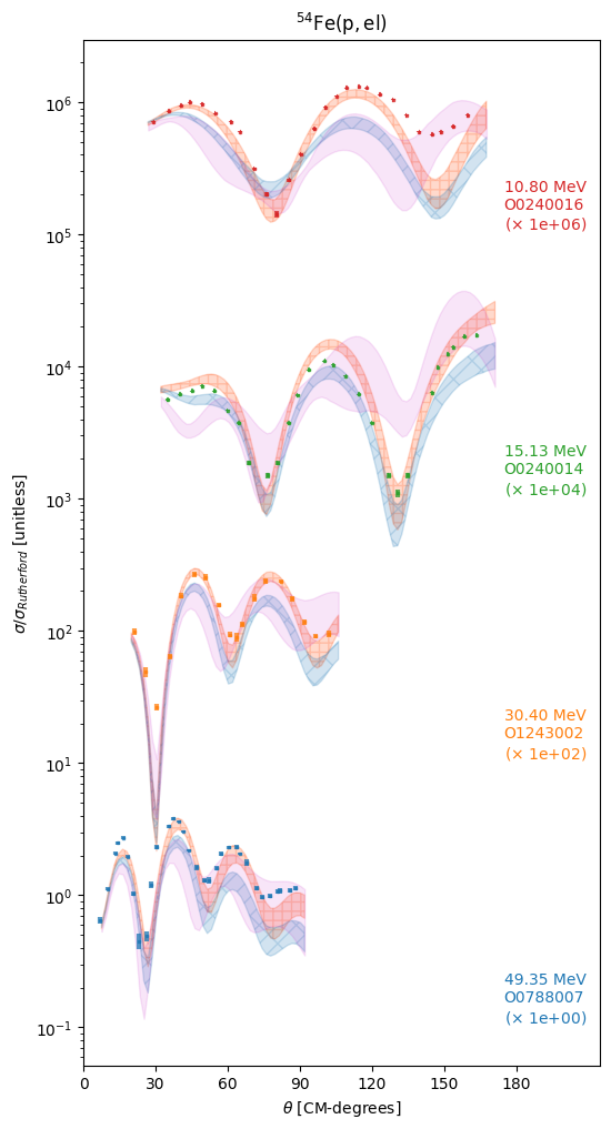
Now that we have our model predictions, lets plot them compared to the experimental data. We will offset each energy for visibility.
Plot the results
 1fig, ax = plt.subplots(1, 1, figsize=(6, 12))
 2offsets = exfor_tools.distribution.AngularDistribution.plot(
 3    all_measurements,
 4    ax,
 5    offsets=100,
 6    data_symbol=list(all_entries.values())[0].data_symbol,
 7    rxn_label=f"${list(all_entries.values())[0].reaction.reaction_latex}$",
 8    label_kwargs={
 9        "label_offset_factor": 0.11,
10        "label_offset": True,
11        "label_exfor": True,
12        "label_xloc_deg": 175,
13        "label_energy_err": False,
14    },
15)
16ax.set_xlim([0, 215])
17
18for i in range(len(all_measurements)):
19    xmin = min([np.min(m.x) for m in all_measurements[i]]) * np.pi / 180
20    xmax = max([np.max(m.x) for m in all_measurements[i]]) * np.pi / 180
21    mask = np.logical_and(angles >= xmin * 0.9, angles < xmax * 1.05)
22
23    # plot models
24    if quantity == "dXS/dA":
25        ax.fill_between(
26            angles[mask] * 180 / np.pi,
27            offsets[i] * kduq_pred_post[i][0][mask] / 1000,
28            offsets[i] * kduq_pred_post[i][1][mask] / 1000,
29            color="#ff4500",
30            hatch="|-|-",
31            alpha=0.2,
32        )
33        ax.fill_between(
34            angles[mask] * 180 / np.pi,
35            offsets[i] * chuq_pred_post[i][0][mask] / 1000,
36            offsets[i] * chuq_pred_post[i][1][mask] / 1000,
37            color="tab:blue",
38            hatch=r"/\/",
39            alpha=0.2,
40        )
41        ax.fill_between(
42            angles[mask] * 180 / np.pi,
43            offsets[i] * wlh_pred_post[i][0][mask] / 1000,
44            offsets[i] * wlh_pred_post[i][1][mask] / 1000,
45            color="m",
46            alpha=0.1,
47        )
48    elif quantity == "dXS/dRuth":
49        ax.fill_between(
50            angles[mask] * 180 / np.pi,
51            offsets[i] * kduq_pred_post[i][0][mask] / solvers[i].rutherford[mask],
52            offsets[i] * kduq_pred_post[i][1][mask] / solvers[i].rutherford[mask],
53            color="#ff4500",
54            hatch="|-|-",
55            alpha=0.2,
56        )
57        ax.fill_between(
58            angles[mask] * 180 / np.pi,
59            offsets[i] * chuq_pred_post[i][0][mask] / solvers[i].rutherford[mask],
60            offsets[i] * chuq_pred_post[i][1][mask] / solvers[i].rutherford[mask],
61            color="tab:blue",
62            hatch=r"/\/",
63            alpha=0.2,
64        )
65        ax.fill_between(
66            angles[mask] * 180 / np.pi,
67            offsets[i] * wlh_pred_post[i][0][mask] / solvers[i].rutherford[mask],
68            offsets[i] * wlh_pred_post[i][1][mask] / solvers[i].rutherford[mask],
69            color="m",
70            alpha=0.1,
71        )
 1fig, ax = plt.subplots(1, 1, figsize=(6, 8))
 2exfor_keys = list(all_entries_Ay.keys())
 3offsets = exfor_tools.distribution.AngularDistribution.plot(
 4    all_measurements_Ay,
 5    ax,
 6    offsets=2,
 7    data_symbol=list(all_entries_Ay.values())[0].data_symbol,
 8    rxn_label=f"${list(all_entries.values())[0].reaction.reaction_latex}$",
 9    draw_baseline=True,
10    baseline_offset=0,
11    log=False,
12    label_kwargs={
13        "label_offset_factor": 0,
14        "label_offset": True,
15        "label_exfor": True,
16        "label_xloc_deg": 180,
17        "label_energy_err": False,
18    },
19)
20ax.set_xlim([0, 215])
21for i in range(len(all_measurements_Ay)):
22    # get x_range
23    xmin = min([np.min(m.x) for m in all_measurements_Ay[i]]) * np.pi / 180
24    xmax = max([np.max(m.x) for m in all_measurements_Ay[i]]) * np.pi / 180
25    mask = np.logical_and(angles >= xmin * 0.8, angles < xmax * 1.2)
26    # plot models
27    ax.fill_between(
28        angles[mask] * 180 / np.pi,
29        offsets[i] + kduq_pred_post_Ay[i][0][mask],
30        offsets[i] + kduq_pred_post_Ay[i][1][mask],
31        color="#ff4500",
32        hatch="|-|-",
33        alpha=0.2,
34    )
35    ax.fill_between(
36        angles[mask] * 180 / np.pi,
37        offsets[i] + chuq_pred_post_Ay[i][0][mask],
38        offsets[i] + chuq_pred_post_Ay[i][1][mask],
39        color="tab:blue",
40        hatch=r"/\/",
41        alpha=0.2,
42    )
43    ax.fill_between(
44        angles[mask] * 180 / np.pi,
45        offsets[i] + wlh_pred_post_Ay[i][0][mask],
46        offsets[i] + wlh_pred_post_Ay[i][1][mask],
47        color="m",
48        alpha=0.1,
49    )