Colab runs this notebook with JITR_QUICK=1 – fewer data points and live points – so the posterior is coarser than the one rendered in the documentation. Drop that line from the setup cell, on a runtime you can keep alive, to reproduce the full result.

Discrete ambiguity in the \(\alpha\) + \(^{48}\)Ca optical potential¶

This is the final notebook in a series of three focusing on \(\alpha\) elastic scattering on Ca isotopes from (Oeschler, 1972):

quickstart introduced the reaction and a least-squares fit
alpha_ca_calibration performed a full Bayesian calibration of \(\alpha\) + \(^{40,44,48}\)Ca elastic scattering at 29 MeV.

We reuse its entire setup - the same data, potential form, error model and likelihood - without repeating the derivations; see that notebook for all of the details.

In this notebook we explore the famous discrete ambiguity of light-ion optical potentials: depths differing by tens of MeV - interior wavefunctions with different numbers of nodes - can produce nearly identical elastic cross sections when the phase between solutions with different numbers of nodes matches up. The discussion in Sec. 9 of the excellent 1971 review article by P E Hodgson, and references therein, go into more detail.

In a Bayesian context, we can understand this discrete ambiguity as a posterior multimodality - multiple distinct regions in parameter space produce distinct cross sections with similar likelihoods of describing the same data. At the end, we will revisit the conclusions of the calibration notebook, in which we chose priors to center on a distinct family, or mode: how do this choice hold up? Is the family we selected there the one the data prefer, and do the quantities we compared between isotopes survive marginalization over the ambiguity?

We don’t want another full analysis that will take an hour to run, so we will a clever trick: the power posterior. This uses a modified form of Bayes’ rule, in which we raise the likelihood \(\ell(\boldsymbol{y} | \alpha)\) to a power (called an inverse temperature) \(\beta\):

(1)¶\[\begin{equation} p_\beta(\alpha | \boldsymbol{y}) = \frac{1}{\mathcal{Z}} \, \left[ \ell ( \boldsymbol{y} | \alpha ) \right]^\beta \, p (\alpha). \end{equation}\]

Here, \(\mathcal{Z} = p(\boldsymbol{y}\) is the Bayesian evidence, and we put a prior \(p(\alpha)\) on the model parameters we are trying to estimate, \(\alpha\). Note that, when \(\beta \rightarrow 1\), we recover standard Bayes, but for \(\beta < 1\), we are choosing to increase the influence of the prior relative to the likelihood, which strongly regularizes the sampling inversion problem.

This is connected to the idea of tempering (or relaxing, or annealing) a likelihood to more efficiently zip past local optima, by increasing the temperature of our sampler. See Swendsen and Wang, 1986 for the physics origins of the idea, Marinari & Parisi (1992) for the generalization to Monte Carlo methods. Gelman & Meng, 1998, and later Nriel & Pettitt, 2008, applied it to Bayesian inference and evidence estimation. Andy Jones has a nice blog post about it too.

We do not need the sharp \(\beta = 1\) posterior to answer the questions we want to answer in this notebook. We are only interested in quickly getting a map in parameter space of where the different modes are, and roughly how they compare. The tempering of the likeliood does not move its peaks, it just broadens each basin and flattens the weights between them, which makes the multimodal landscape vastly cheaper to explore. The result is a survey of the discrete ambiguity that runs in a few minutes rather than hours.

In a production calibration setting, one might actually want to do this first rather than last. Getting quickly to a rough map of the landscape of multimodality allows us to think about what modes are interesting to our problem (e.g. on physical grounds, or to make an apples-apples comparison to previous work), and adjust our full calibration accordingly.

import os

# keep every process single-threaded: we will parallelize over likelihood
# evaluations with multiprocessing below, and nested BLAS/numba threads would
# oversubscribe the CPU. Must be set before numpy/jitr are imported.
os.environ.setdefault("OMP_NUM_THREADS", "1")
os.environ.setdefault("OPENBLAS_NUM_THREADS", "1")
os.environ.setdefault("MKL_NUM_THREADS", "1")
os.environ.setdefault("NUMBA_NUM_THREADS", "1")

import numpy as np
import pandas as pd
from matplotlib import pyplot as plt
from scipy import stats

# JITR_QUICK=1 runs a cut-down version of the notebook (fewer data points and live points) for CI
QUICK = os.environ.get("JITR_QUICK", "0") == "1"

Set up the reaction, data and solver¶

Exactly as in the calibration notebook.

from jitr.reactions.reaction import Reaction

targets = {"Ca48": (48, 20)}
alpha = (4, 2)
reactions = {
    key: Reaction(target=target, projectile=alpha, process="El")
    for key, target in targets.items()
}

# calculate kinematics for a given lab energy
energy_lab = 29
kinematics = {
    key: reaction.kinematics(energy_lab) for key, reaction in reactions.items()
}

df = pd.read_csv("./alpha_ca_ratio_ruth.csv")
df = df[df["target"] == "Ca48"]
if QUICK:
    df = df.iloc[::4]
data = {
    key: {
        "x": group["angle_cm_deg"].to_numpy(),
        "y": group["ratio_to_rutherford"].to_numpy(),
    }
    for key, group in df.groupby("target")
}
colors = {"Ca48": "#FF9900"}
isotope_label = {key: rf"$^{{{A}}}$Ca" for key, (A, Z) in targets.items()}

from jitr.rmatrix import Solver as SolverKernel
from jitr.utils import utils
from jitr.xs import elastic

lmax = 60


def build_solver(key, angles_deg):
    A, Z = targets[key]
    interaction_range_fm = 1.2 * (A ** (1 / 3) + 4 ** (1 / 3)) + 2
    channel_radius_dimensionless = utils.suggested_dimensionless_channel_radius(
        interaction_range_fm, kinematics[key].k
    )
    channel_radius = channel_radius_dimensionless / kinematics[key].k
    N = utils.suggested_basis_size(channel_radius_dimensionless, zeros_per_node=8)
    print(
        f"Compiling solver for {reactions[key]} at {energy_lab} MeV: "
        f"channel radius {channel_radius:1.2f} fm, {N} nodes, {lmax} partial waves"
    )
    return elastic.DifferentialWorkspace.build_from_system(
        reaction=reactions[key],
        kinematics=kinematics[key],
        channel_radius_fm=channel_radius,
        solver=SolverKernel(N),
        lmax=lmax,
        angles=np.deg2rad(angles_deg),
    )


solvers = {key: build_solver(key, data[key]["x"]) for key in targets}

Compiling solver for 48-Ca(alpha,el) at 29 MeV: channel radius 11.15 fm, 64 nodes, 60 partial waves

# jit warmup - do this before forking worker processes later so they inherit compiled code
for solver in solvers.values():
    _ = solver.xs(central_potential=np.zeros_like(solver.radial_grid()))

The interaction¶

The same seven-parameter potential as the calibration notebook.

from jitr.optical_potentials.potential_forms import (
    coulomb_charged_sphere as coulomb,
)
from jitr.optical_potentials.potential_forms import (
    woods_saxon_prime_safe as wsp,
)
from jitr.optical_potentials.potential_forms import (
    woods_saxon_safe as ws,
)


def U_central(r, Vv, Wv, Ws, Rv, av, Rw, aw):
    return (
        -Vv * ws(r, Rv, av)
        - 1j * Wv * ws(r, Rw, aw)
        - 1j * Ws * (-4 * aw) * wsp(r, Rw, aw)
    )


def calculate_xs_ratio(theta, key):
    """Ratio to Rutherford on the data angles of `key` for optical model parameters `theta`."""
    solver = solvers[key]
    reaction = reactions[key]
    # each solver has its own radial quadrature grid (it depends on the channel radius)
    rgrid = solver.radial_grid()
    Vv, Wv, Ws, rv, av, rw, aw = theta
    A_factor = reaction.target.A ** (1 / 3)
    Zz = reaction.target.Z * reaction.projectile.Z
    xs = solver.xs(
        central_potential=U_central(
            rgrid, Vv, Wv, Ws, rv * A_factor, av, rw * A_factor, aw
        ),
        coulomb_potential=coulomb(rgrid, Zz, 1.3 * A_factor),
    )
    return xs.dsdo / solver.rutherford


names = ["Vv", "Wv", "Ws", "rv", "av", "rw", "aw"]
labels = [r"$V$", r"$W_v$", r"$W_s$", r"$r_v$", r"$a_v$", r"$r_w$", r"$a_w$"]
n_omp = len(names)

The error model and likelihood¶

Identical to alpha_ca_calibration.ipynb: a relative error \(s\) uncorrelated from point to point plus a relative error \(b\) common to all points, evaluated exactly in log space at \(O(N)\) cost. The cell below is copied verbatim from there - see that notebook for the derivation.

ERR_NAMES = ["log_s", "log_b"]
ERR_LABELS = [r"$s$", r"$b$"]
n_err = len(ERR_NAMES)
ndim = n_omp + n_err
all_labels = labels + ERR_LABELS


def unpack(theta):
    return theta[:n_omp], np.exp(theta[n_omp:])  # potential parameters, (s, b)


def log_likelihood(theta, key):
    omp, (s, b) = unpack(theta)
    y = data[key]["y"]
    if np.any(omp[3:] <= 0):  # radii and diffusenesses must be positive
        return -1e300
    f_pred = calculate_xs_ratio(omp, key)  # f_i = f(theta_i; alpha)
    if np.any(f_pred <= 0) or not np.all(np.isfinite(f_pred)):
        return -1e300
    log_residuals = np.log(y) - np.log(f_pred)  # r_i = log y_i - log f_i
    n_pts = log_residuals.size

    # Sigma^log = d I + beta 11^T - homoscedastic, because both error terms are relative
    common_log_var = np.log1p(b**2)  # beta, added to every entry by the shared factor B
    point_log_var = np.log1p(s**2 / (1 + b**2))  # d, from the independent factors A_i

    # Sherman-Morrison:
    # r^T (Sigma^log)^-1 r = (r^T r)/d - beta (1^T r)^2 / (d (d + N beta))
    shared_term_denom = point_log_var + n_pts * common_log_var  # d + N beta
    mahalanobis = (
        log_residuals @ log_residuals / point_log_var
        - common_log_var
        * np.sum(log_residuals) ** 2
        / (point_log_var * shared_term_denom)
    )
    # matrix determinant lemma: det(Sigma^log) = d^(N-1) (d + N beta)
    log_det = (n_pts - 1) * np.log(point_log_var) + np.log(shared_term_denom)

    jacobian = -np.sum(np.log(y))  # density for y, not log y
    return -0.5 * (mahalanobis + log_det + n_pts * np.log(2 * np.pi)) + jacobian


def predictive_draw(s, b, f_pred, rng):
    """One synthetic data set drawn from the error model around the model prediction f_pred."""
    # log y_i = log f_i + independent relative scatter (A_i) + one shared relative shift (B)
    log_noise = (
        np.sqrt(np.log1p(s**2 / (1 + b**2))) * rng.normal(size=f_pred.shape)
        + np.sqrt(np.log1p(b**2)) * rng.normal()
    )
    return f_pred * np.exp(log_noise)

Prior¶

Independent uniform priors over loose physical bounds. The real depth spans \(V \in [50, 300]\) MeV - deep enough to hold several node-count families - the absorptive depths span \([0, 60]\) MeV, and the geometries cover the physically sensible window for \(\alpha\)-nucleus scattering. The error scales keep the same log-uniform priors as the calibration notebook.

omp_prior = {
    "Ca48": [
        stats.uniform(50, 250),  # V  in [50, 300] MeV
        stats.uniform(0, 60),  # Wv in [0, 60] MeV
        stats.uniform(0, 60),  # Ws in [0, 60] MeV
        stats.uniform(1.0, 0.7),  # rv in [1.0, 1.7] A^1/3 fm
        stats.uniform(0.4, 0.5),  # av in [0.4, 0.9] fm
        stats.uniform(1.0, 0.8),  # rw in [1.0, 1.8] A^1/3 fm
        stats.uniform(0.15, 0.75),  # aw in [0.15, 0.9] fm
    ]
}

err_prior = [
    stats.loguniform(5e-2, 2.0),  # s: relative, point-to-point independent error
    stats.loguniform(5e-2, 2.0),  # b: relative, fully correlated error
]


def prior_transform(u, key):
    omp = np.array([p.ppf(ui) for p, ui in zip(omp_prior[key], u[:n_omp], strict=True)])
    err = [np.log(p.ppf(ui)) for p, ui in zip(err_prior, u[n_omp:], strict=True)]
    return np.concatenate([omp, err])

Sampling the tempered posterior¶

The length of a nested sampling run scales with the information gained going from the prior to the posterior, and with the number of live points needed to keep every mode populated. Tempering attacks the first factor directly: with \(T = 4\), the tempered posterior carries far less information than the full one, so the run terminates quickly, while each family - \(\sim\) 2 MeV wide in \(V\) at \(\beta = 1\) - broadens by roughly \(\beta^{-1/2} = 2\times\), still far narrower than the \(\sim\) 40 MeV spacing between families. (Temper too hard and the families smear into the prior; \(T \sim 10\) already washes out the valley between the two shallowest families here.) We also shorten dynesty’s random walks: each replacement step needs fewer proposals on a broad, flattened target, which is where most of the run time goes.

import multiprocessing
from functools import partial

import dynesty

temperature = 4
beta_temper = 1 / temperature


def log_likelihood_tempered(theta, key):
    return beta_temper * log_likelihood(theta, key)


n_workers = min(4, os.cpu_count())
nlive = 100 if QUICK else 300
dlogz = 5.0 if QUICK else 1.0
print(
    f"Using {n_workers} worker processes, nlive={nlive}, dlogz={dlogz}, temperature={temperature}"
)

Using 4 worker processes, nlive=300, dlogz=1.0, temperature=4

%%time
results = {}
with multiprocessing.get_context("fork").Pool(n_workers) as pool:
    for key in targets:
        sampler = dynesty.NestedSampler(
            partial(log_likelihood_tempered, key=key),
            partial(prior_transform, key=key),
            ndim,
            nlive=nlive,
            sample="rwalk",
            walks=12,  # a broad, tempered target needs fewer random-walk steps per replacement
            pool=pool,
            queue_size=n_workers,
            rstate=np.random.default_rng(0),
        )
        sampler.run_nested(dlogz=dlogz, print_progress=False)
        results[key] = sampler.results
        print(
            f"{key}: tempered log Z = {results[key].logz[-1]:.2f} +/- {results[key].logzerr[-1]:.2f}, "
            f"{int(np.sum(results[key].ncall))} calls, efficiency {results[key].eff:.1f} %"
        )

Ca48: tempered log Z = 200.99 +/- 0.56, 78043 calls, efficiency 8.9 %
CPU times: user 10.9 s, sys: 722 ms, total: 11.7 s
Wall time: 16min 28s

rng = np.random.default_rng(42)
posterior_samples = {key: results[key].samples_equal(rstate=rng) for key in targets}
print(f"{len(posterior_samples['Ca48'])} equally weighted posterior samples")

6929 equally weighted posterior samples

The posterior¶

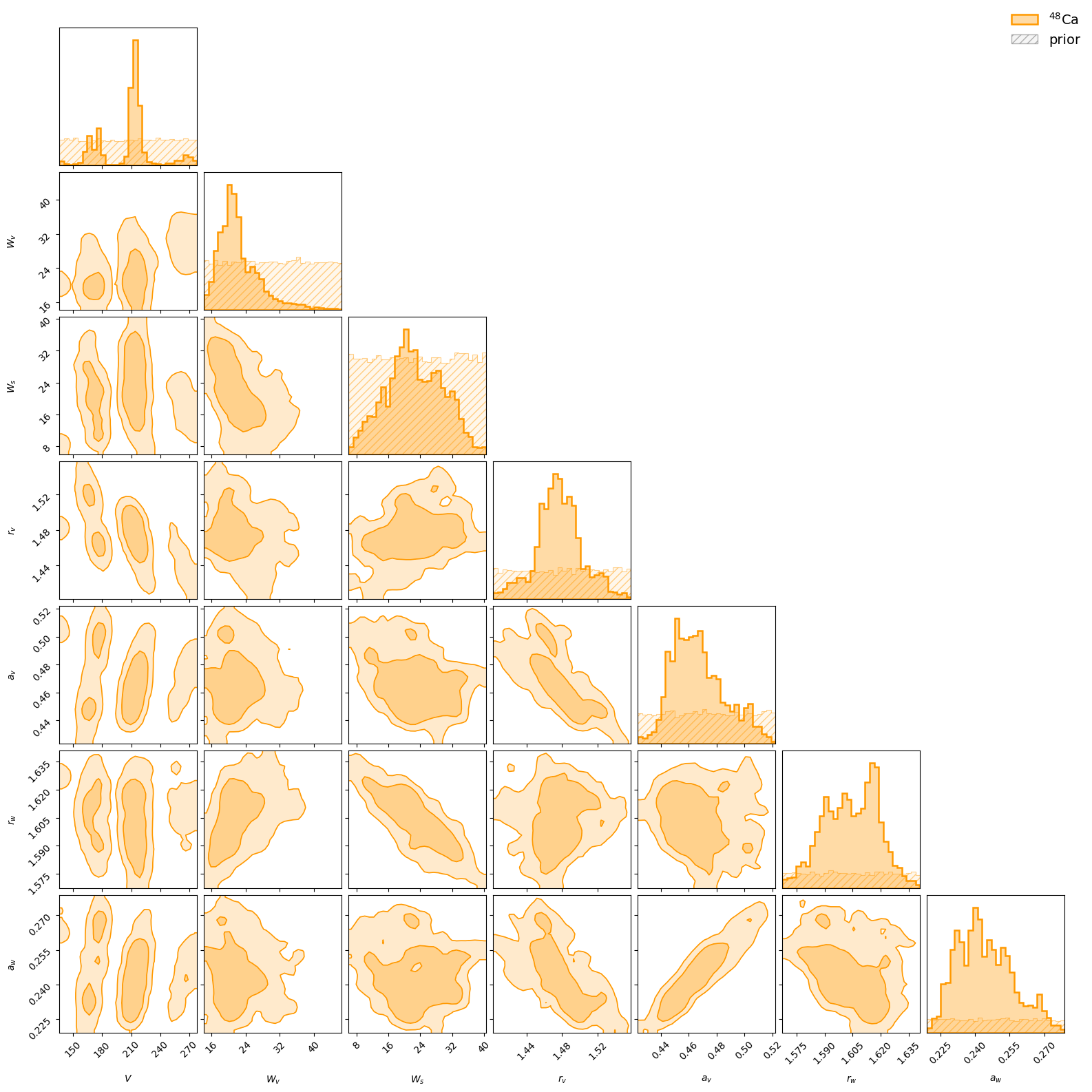
The corner plot of the potential parameters now shows several well separated islands - each one a discrete family. The hatched histograms on the diagonal are the priors: flat, and tiny compared to the posterior density, so everything below is driven by the likelihood.

Remember that the width of each island is inflated by the tempering; at \(\beta = 1\) each family is \(\sim\) 3 times narrower.

import corner
from matplotlib.colors import to_rgba
from matplotlib.patches import Patch


def corner_overlay(samples, labels, keys, priors=None, ranges=None, **kwargs):
    """Overlay corner plots for several data sets with a common range.

    Ranges are driven by the posteriors (central 99%), so the panels zoom in on
    them; `priors` (dict key -> (n, ndim) sample array) are drawn on the 1D panels
    only, as hatched histograms on the full-prior density scale - where the
    posterior is likelihood-dominated they appear as small, nearly flat slices.
    """
    if ranges is None:
        allsamples = np.vstack([samples[key] for key in keys])
        ranges = list(
            zip(
                np.percentile(allsamples, 0.5, axis=0),
                np.percentile(allsamples, 99.5, axis=0),
                strict=True,
            )
        )
    npanel = len(ranges)
    fig = None
    for key in keys:
        c = colors[key]
        fig = corner.corner(
            samples[key],
            labels=labels,
            color=c,
            fig=fig,
            range=ranges,
            bins=30,
            smooth=1.0,
            plot_datapoints=False,
            plot_density=False,
            levels=(0.68, 0.95),
            fill_contours=True,
            contourf_kwargs={
                "colors": [(0, 0, 0, 0), to_rgba(c, 0.2), to_rgba(c, 0.45)]
            },
            contour_kwargs={"colors": [to_rgba(c, 1.0)], "linewidths": 1.2},
            hist_kwargs={
                "density": True,
                "histtype": "stepfilled",
                "facecolor": to_rgba(c, 0.35),
                "edgecolor": to_rgba(c, 1.0),
                "linewidth": 1.8,
            },
            **kwargs,
        )
    if priors is not None:
        axes = np.array(fig.axes).reshape(npanel, npanel)
        for key in keys:
            c = colors[key]
            for i in range(npanel):
                draws = priors[key][:, i]
                lo, hi = ranges[i]
                counts, edges = np.histogram(draws, bins=30, range=(lo, hi))
                density = 3 * counts / (len(draws) * np.diff(edges))
                axes[i, i].stairs(
                    density,
                    edges,
                    fill=True,
                    facecolor=to_rgba(c, 0.08),
                    edgecolor=to_rgba(c, 0.45),
                    hatch="///",
                    linewidth=0.8,
                )
    handles = [
        Patch(
            facecolor=to_rgba(colors[key], 0.35),
            edgecolor=colors[key],
            linewidth=1.8,
            label=isotope_label[key],
        )
        for key in keys
    ]
    if priors is not None:
        handles.append(
            Patch(
                facecolor=to_rgba("gray", 0.08),
                edgecolor=to_rgba("gray", 0.6),
                hatch="///",
                label="prior",
            )
        )
    fig.legend(handles=handles, loc="upper right", fontsize=14, framealpha=0)
    return fig


n_prior_draws = 40000
prior_rng = np.random.default_rng(7)
omp_prior_draws = {
    key: np.column_stack(
        [p.rvs(n_prior_draws, random_state=prior_rng) for p in omp_prior[key]]
    )
    for key in targets
}

omp_samples = {key: posterior_samples[key][:, :n_omp] for key in targets}
fig = corner_overlay(omp_samples, labels, list(targets), priors=omp_prior_draws)
plt.show()

../../_images/eb7a1e2bfe2d5cdb47de3e609ff5086a75b0083e06bacd88c5518e2ca84e0da0.png

Decomposing the posterior into modes¶

The modes are cleanly separated in \(V\), so we can split the samples at the minima of a kernel density estimate of the marginal posterior of \(V\), and summarize each family separately: its posterior mass (the probability, given data, prior, and model, that this family is the right one), its parameters, and its volume integrals per nucleon pair,

\[ \frac{J_U}{4A} = \frac{4\pi}{4A}\int_0^\infty U(r)\, r^2\, dr . \]

from scipy.stats import gaussian_kde


def volume_integral_per_nucleon(samples, key):
    """(J_V + i J_W) / (4 A) [MeV fm^3] for each posterior sample."""
    A = targets[key][0]
    r = np.linspace(0, 20, 2000)
    out = np.zeros(len(samples), dtype=complex)
    for i, (Vv, Wv, Ws, rv, av, rw, aw) in enumerate(samples[:, :n_omp]):
        Rv = rv * A ** (1 / 3)
        Rw = rw * A ** (1 / 3)
        out[i] += np.trapezoid(Vv * ws(r, Rv, av) * r**2, r)
        out[i] += 1j * np.trapezoid(
            (Wv * ws(r, Rw, aw) + Ws * (-4 * aw) * wsp(r, Rw, aw)) * r**2, r
        )
    return 4 * np.pi / (4 * A) * out


def summarize(samples):
    q = np.percentile(samples, [16, 50, 84], axis=0)
    return [f"{m:.3g} [{lo:.3g}, {hi:.3g}]" for lo, m, hi in q.T]


# split the samples at the local minima of a KDE of the V marginal
v_samples = posterior_samples["Ca48"][:, 0]
# smooth by at least ~5 MeV: genuine families are ~40 MeV apart, while
# finite-sampling noise fragments a single family into sub-MeV wiggles
bw = max(len(v_samples) ** (-0.2), 5.0 / np.std(v_samples))
kde = gaussian_kde(v_samples, bw_method=bw)
v_grid = np.linspace(v_samples.min(), v_samples.max(), 1000)
density = kde(v_grid)
is_valley = (density[1:-1] < density[:-2]) & (density[1:-1] < density[2:])
cuts = v_grid[1:-1][is_valley]
mode_index = np.digitize(v_samples, cuts)
mode_weights = np.array([np.mean(mode_index == m) for m in range(len(cuts) + 1)])
modes = [m for m in np.argsort(mode_weights)[::-1] if mode_weights[m] >= 0.01]
modes = sorted(modes, key=lambda m: np.median(v_samples[mode_index == m]))  # order by V
print(
    f"{len(modes)} modes hold at least 1% of the posterior mass (of {len(cuts) + 1} candidates)"
)

mode_samples = {m: posterior_samples["Ca48"][mode_index == m] for m in modes}
mode_jv = {m: volume_integral_per_nucleon(mode_samples[m], "Ca48") for m in modes}
mode_names = {
    m: f"mode {i} ({100 * mode_weights[m]:.0f}% tempered mass)"
    for i, m in enumerate(modes)
}

# which family does the full (untempered) likelihood prefer? The sampler stored
# beta * log L for every point it visited, so divide beta back out and compare maxima
raw_mode_index = np.digitize(results["Ca48"].samples[:, 0], cuts)
best_logl = {
    m: results["Ca48"].logl[raw_mode_index == m].max() / beta_temper for m in modes
}
delta_best_logl = {m: best_logl[m] - max(best_logl.values()) for m in modes}

pd.DataFrame(
    {
        mode_names[m]: summarize(
            np.column_stack(
                [
                    mode_samples[m][:, :n_omp],
                    np.exp(mode_samples[m][:, n_omp:]),
                    mode_jv[m].real,
                    mode_jv[m].imag,
                ]
            )
        )
        + [f"{delta_best_logl[m]:.1f}"]
        for m in modes
    },
    index=names
    + [n.removeprefix("log_") for n in ERR_NAMES]
    + ["J_V/4A [MeV fm^3]", "J_W/4A [MeV fm^3]", "max log L - best (untempered)"],
)

4 modes hold at least 1% of the posterior mass (of 5 candidates)

	mode 0 (1% tempered mass)	mode 1 (25% tempered mass)	mode 2 (65% tempered mass)	mode 3 (8% tempered mass)
Vv	138 [135, 140]	171 [164, 178]	214 [210, 218]	267 [257, 274]
Wv	20.1 [19.4, 34.1]	20.1 [17.8, 23.6]	21.2 [17.9, 25.6]	28 [25.6, 34.5]
Ws	8.59 [7.69, 16.9]	20.7 [12.3, 27.6]	23.8 [17.3, 31.7]	18 [13, 23.7]
rv	1.48 [1.48, 1.54]	1.49 [1.46, 1.53]	1.48 [1.46, 1.49]	1.43 [1.42, 1.46]
av	0.503 [0.463, 0.511]	0.478 [0.445, 0.503]	0.463 [0.45, 0.477]	0.473 [0.454, 0.487]
rw	1.63 [1.61, 1.63]	1.61 [1.59, 1.62]	1.6 [1.59, 1.62]	1.61 [1.6, 1.62]
aw	0.262 [0.251, 0.273]	0.249 [0.231, 0.268]	0.241 [0.232, 0.253]	0.244 [0.233, 0.256]
s	0.482 [0.466, 0.555]	0.532 [0.486, 0.589]	0.503 [0.47, 0.558]	0.526 [0.497, 0.562]
b	0.0911 [0.081, 0.129]	0.136 [0.0709, 0.25]	0.138 [0.0899, 0.29]	0.128 [0.0735, 0.254]
J_V/4A [MeV fm^3]	515 [505, 533]	637 [625, 654]	774 [761, 785]	893 [877, 910]
J_W/4A [MeV fm^3]	112 [110, 194]	132 [124, 153]	144 [137, 157]	162 [153, 194]
max log L - best (untempered)	-14.4	-4.2	0.0	-7.0

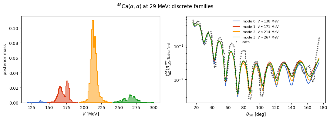
The families are far apart in parameter space, but produce nearly the same cross section - that is what makes this a genuine discrete ambiguity rather than a poorly converged fit. Below, the marginal posterior of \(V\) colored by mode, and the median model curve of each mode against the data.

mode_colors = {
    m: c
    for m, c in zip(
        modes,
        ["#3366CC", "#DC3912", "#FF9900", "#109618", "#990099", "#0099C6"],
        strict=False,
    )
}

fig, axes = plt.subplots(1, 2, figsize=(11, 4))
for i, m in enumerate(modes):
    axes[0].hist(
        mode_samples[m][:, 0],
        bins=30,
        weights=np.full(len(mode_samples[m]), 1.0 / len(v_samples)),
        facecolor=to_rgba(mode_colors[m], 0.5),
        edgecolor=mode_colors[m],
        linewidth=1.5,
        histtype="stepfilled",
    )
    theta_median = np.median(mode_samples[m][:, :n_omp], axis=0)
    axes[1].plot(
        data["Ca48"]["x"],
        calculate_xs_ratio(theta_median, "Ca48"),
        color=mode_colors[m],
        label=rf"mode {i}: $V \approx {theta_median[0]:.0f}$ MeV",
    )
axes[0].set_xlabel(r"$V$ [MeV]")
axes[0].set_ylabel("posterior mass")
axes[1].plot(
    data["Ca48"]["x"],
    data["Ca48"]["y"],
    ".",
    color="k",
    alpha=0.5,
    markersize=4,
    label="data",
)
axes[1].set_yscale("log")
axes[1].set_xlabel(r"$\theta_{cm}$ [deg]")
axes[1].set_ylabel(
    r"$(\frac{d\sigma}{d\Omega}) / (\frac{d\sigma}{d\Omega})_\text{Rutherford}$"
)
axes[1].legend(framealpha=0, fontsize=8)
fig.suptitle(r"$^{48}$Ca($\alpha,\alpha$) at 29 MeV: discrete families")
plt.tight_layout()
plt.show()

../../_images/04175e9d215d9c8cbc275cd851e561c735780f02de32bb8f2a528e60130fec18.png

How do the calibration conclusions hold up?¶

The data support a ladder of discrete families. With loose physical bounds, four modes survive, at \(V \approx 138, 171, 214\) and \(267\) MeV - spaced by the characteristic \(\sim 40\)-\(50\) MeV of the node-count ambiguity, with real volume integrals climbing in steps of \(\sim 120\) MeV fm\(^3\). Their cross sections are nearly degenerate over most of the angular range and separate only at the most backward angles, which is precisely what makes this an ambiguity: no amount of forward-angle data will resolve it.

The family selected in the calibration notebook is the one the data prefer. The \(V \approx 214\) window carries both the largest tempered mass (65%) and the highest untempered best-fit likelihood - the runner-up at \(V \approx 171\) sits \(\sim 4\) units of log-likelihood lower, \(V \approx 267\) sits \(\sim 7\) lower, and \(V \approx 138\) is out of the running. So the prior choice made there - selecting the deep family near \(V \approx 205\) - agrees with what a much more expensive, wide-open search recovers.

It is worth stating that, in general, this sort of analysis is really powerful as a first step, to get a rough map of the posterior landscape before moving to full calibration.