Compare global optical-potential radial forms
This notebook compares the radial structure of several built-in global optical potentials. It is useful when you want a quick visual sense of how the parameterizations differ before running a larger study.
1import numpy as np
1from matplotlib import pyplot as plt
1from jitr.reactions import ElasticReaction
1from jitr.optical_potentials import chuq, kduq, wlh
1neutron = (1, 0)
2proton = (1, 1)
1target = (208, 82)
2projectile = neutron
3energy_lab = 20
4rxn = ElasticReaction(target=target, projectile=projectile)
 1samples = {
 2    "KDUQ": kduq.get_samples(projectile),
 3    "CHUQ": chuq.get_samples(),
 4    "WLH": wlh.get_samples(projectile),
 5}
 6models = {
 7    "KDUQ": kduq.KDUQ(projectile),
 8    "WLH": wlh.WLH(projectile),
 9    "CHUQ": chuq.CHUQ(),
10}
 1kinematics = rxn.kinematics(energy_lab)
 2r = np.linspace(0.1, 15.0, 300)
 3
 4
 5def complex_pctl(values, pctls):
 6    q_real = np.percentile(values.real, pctls, axis=0)
 7    q_imag = np.percentile(values.imag, pctls, axis=0)
 8    return q_real[0] + 1j * q_imag[0], q_real[1] + 1j * q_imag[1]
 9
10
11kinematics
ChannelKinematics(Elab=20, Ecm=19.903449469680808, mu=np.float64(954.6903694711453), k=np.float64(0.982788204101379), eta=np.float64(0.0))
 1def generate_potential_bands(omp, samples, pctls=None):
 2    if pctls is None:
 3        pctls = [16, 84]
 4    U_central = np.zeros((len(samples), r.size), dtype=complex)
 5    U_so = np.zeros((len(samples), r.size), dtype=complex)
 6
 7    for i, x in enumerate(samples):
 8        central_term, so_term, _ = omp(r, rxn, kinematics, *x)
 9        U_central[i, :] = central_term
10        U_so[i, :] = so_term
11
12    l_so, h_so = complex_pctl(U_so, pctls)
13    l_c, h_c = complex_pctl(U_central, pctls)
14    return (l_c, h_c), (l_so, h_so)
1potential_bands = {
2    key: generate_potential_bands(models[key], samples[key])
3    for key in ["KDUQ", "CHUQ", "WLH"]
4}
1colors = {"KDUQ": "tab:orange", "CHUQ": "tab:blue", "WLH": "tab:green"}
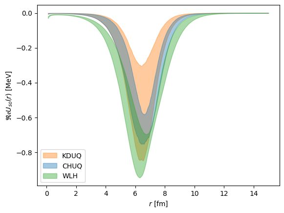
1for key, (_, bounds) in potential_bands.items():
2    l, h = bounds[0], bounds[1]
3    plt.fill_between(r, l.real, h.real, label=key, alpha=0.4, color=colors[key])
4
5plt.legend()
6plt.ylabel(r"$\mathfrak{Re} U_{so}(r)$ [MeV]")
7plt.xlabel(r"$r$ [fm]")
Text(0.5, 0, '$r$ [fm]')
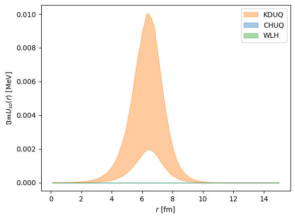
1for key, (_, bounds) in potential_bands.items():
2    l, h = bounds[0], bounds[1]
3    plt.fill_between(r, l.imag, h.imag, label=key, alpha=0.4, color=colors[key])
4
5plt.legend()
6plt.ylabel(r"$\mathfrak{Im} U_{so}(r)$ [MeV]")
7plt.xlabel(r"$r$ [fm]")
Text(0.5, 0, '$r$ [fm]')
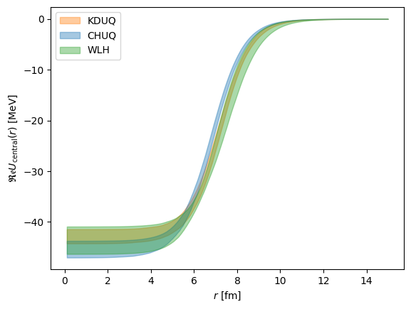
1for key, (bounds, _) in potential_bands.items():
2    l, h = bounds[0], bounds[1]
3    plt.fill_between(r, l.real, h.real, label=key, alpha=0.4, color=colors[key])
4
5plt.legend()
6plt.ylabel(r"$\mathfrak{Re} U_{\text{central}}(r)$ [MeV]")
7plt.xlabel(r"$r$ [fm]")
Text(0.5, 0, '$r$ [fm]')
1for key, (bounds, _) in potential_bands.items():
2    l, h = bounds[0], bounds[1]
3    plt.fill_between(r, l.imag, h.imag, label=key, alpha=0.4, color=colors[key])
4
5plt.legend()
6plt.ylabel(r"$\mathfrak{Im} U_{\text{central}}(r)$ [MeV]")
7plt.xlabel(r"$r$ [fm]")
Text(0.5, 0, '$r$ [fm]')
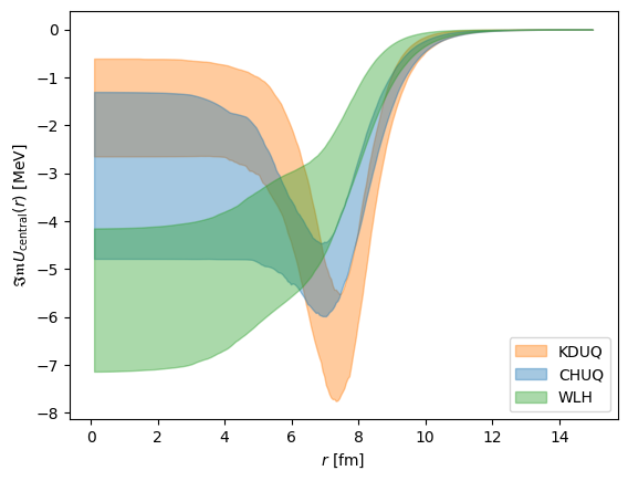
Compare the imaginary components
Notice only one potential has an imaginary spin orbit term, and that WLH is much less surface peaked than the other two.