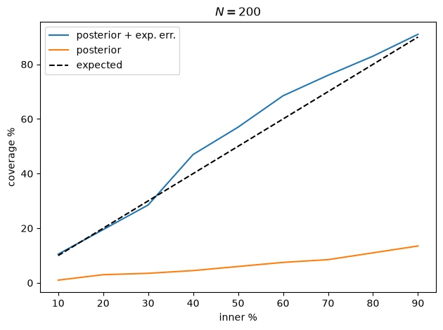
Large N implies overconfidence? Do we need to re-scale the Likelihood?#
from collections import OrderedDict
import corner
import numpy as np
from matplotlib import pyplot as plt
from scipy import stats
from scipy.stats import norm
import rxmc
Using database version X4-2024-12-31 located in: /home/kyle/db/exfor/unpack_exfor-2024/X4-2024-12-31
true_params = OrderedDict(
    [
        ("m", 2),
        ("b", 4),
    ]
)
rng = np.random.default_rng(42)
noise = 0.05
N = 200
# x_data = np.sort(np.random.rand(N))
x_data = np.linspace(0, 1, N)
y_true = true_params["m"] * x_data + true_params["b"]
y_err = np.array([rng.normal(0, noise * y) for y in y_true])
y_data = y_true + y_err

reported_stat_err = noise * y_data
class LinearModel(rxmc.physical_model.PhysicalModel):
    def __init__(self):
        params = [
            rxmc.params.Parameter("m", float, "no-units"),
            rxmc.params.Parameter("b", float, "y-units"),
        ]
        super().__init__(params)

    def evaluate(self, observation, m, b):
        return self.y(observation.x, m, b)

    def y(self, x, m, b):
        # useful to have a function hat takes in an array-like x
        # rather than an Observation, e.g. for plotting
        return m * x + b
prior_mean = OrderedDict(
    [
        ("m", 1),
        ("b", 4),
    ]
)
prior_std_dev = OrderedDict(
    [
        ("m", 0.1),
        ("b", 0.5),
    ]
)
covariance = np.diag(list(prior_std_dev.values())) ** 2
mean = np.array(list(prior_mean.values()))
prior_distribution = stats.multivariate_normal(mean, covariance)
mean
array([1, 4])
my_model = LinearModel()
observation = rxmc.observation.Observation(
    x=x_data,
    y=y_data,
    y_stat_err=y_true * noise,
)
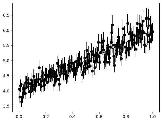
plt.errorbar(
    x_data,
    y_data,
    noise * y_data,
    color="k",
    marker="o",
    linestyle="none",
    label="experiment",
)
plt.plot(x_data, y_true, "k--", label="truth")
[<matplotlib.lines.Line2D at 0x74ab31533c80>]
likelihood = rxmc.likelihood_model.GaussianLikelihood()
evidence = rxmc.evidence.Evidence(
    [
        rxmc.constraint.Constraint(
            [observation],
            my_model,
            likelihood,
        )
    ],
)
evidence_scaled = rxmc.evidence.Evidence(
    [
        rxmc.constraint.Constraint(
            [observation],
            my_model,
            likelihood,
        )
    ],
    weights=np.array([2 / N]),
)
The same tempering as a config-level knob#
Evidence(weights=...) tempers the likelihood per constraint;
CalibrationConfig(likelihood_scaling=...) tempers the whole likelihood.
For a single constraint they are two spellings of the same thing — and both
propagate consistently into the Gibbs conditionals
(CalibrationConfig.conditional_posterior applies
likelihood_scaling * weight to the marginal likelihood, with the prior
untouched), so the tempered joint is what every sampling block targets.
model_config = rxmc.config.ParameterConfig(
    params=my_model.params,
    prior=prior_distribution,
    initial_proposal_distribution=prior_distribution,
)

config_scaling = rxmc.config.CalibrationConfig(
    evidence=rxmc.evidence.Evidence(
        [rxmc.constraint.Constraint([observation], my_model, likelihood)]
    ),
    model_config=model_config,
    likelihood_scaling=2 / N,
)
config_weights = rxmc.config.CalibrationConfig(
    evidence=evidence_scaled,
    model_config=model_config,
)

x_test = np.array([2.0, 4.0])
print(f"likelihood_scaling = 2/N : {config_scaling.log_likelihood(x_test):.6f}")
print(f"Evidence weights = [2/N] : {config_weights.log_likelihood(x_test):.6f}")
likelihood_scaling = 2/N : 0.173502
Evidence weights = [2/N] : 0.173502
def proposal_distribution(x, rng):
    return stats.multivariate_normal.rvs(
        mean=x, cov=prior_distribution.cov / 100, random_state=rng
    )
walker_scaled = rxmc.walker.Walker(
    rxmc.param_sampling.BatchedAdaptiveMetropolisSampler(
        params=my_model.params,
        starting_location=prior_distribution.mean,
        prior=prior_distribution,
        initial_proposal_cov=prior_distribution.cov / 100,
    ),
    evidence_scaled,
)
walker = rxmc.walker.Walker(
    rxmc.param_sampling.BatchedAdaptiveMetropolisSampler(
        params=my_model.params,
        starting_location=prior_distribution.mean,
        prior=prior_distribution,
        initial_proposal_cov=prior_distribution.cov / 100,
    ),
    evidence,
)
%%time
walker_scaled.walk(n_steps=10000, burnin=1000, batch_size=500)
Burn-in batch 1/2 completed, 500 steps.
Burn-in batch 2/2 completed, 500 steps.
Batch: 1/20 completed, 500 steps.
  Model parameter acceptance fraction: 0.390
Batch: 2/20 completed, 500 steps.
  Model parameter acceptance fraction: 0.364
Batch: 3/20 completed, 500 steps.
  Model parameter acceptance fraction: 0.336
Batch: 4/20 completed, 500 steps.
  Model parameter acceptance fraction: 0.360
Batch: 5/20 completed, 500 steps.
  Model parameter acceptance fraction: 0.394
Batch: 6/20 completed, 500 steps.
  Model parameter acceptance fraction: 0.386
Batch: 7/20 completed, 500 steps.
  Model parameter acceptance fraction: 0.390
Batch: 8/20 completed, 500 steps.
  Model parameter acceptance fraction: 0.358
Batch: 9/20 completed, 500 steps.
  Model parameter acceptance fraction: 0.342
Batch: 10/20 completed, 500 steps.
  Model parameter acceptance fraction: 0.384
Batch: 11/20 completed, 500 steps.
  Model parameter acceptance fraction: 0.338
Batch: 12/20 completed, 500 steps.
  Model parameter acceptance fraction: 0.370
Batch: 13/20 completed, 500 steps.
  Model parameter acceptance fraction: 0.368
Batch: 14/20 completed, 500 steps.
  Model parameter acceptance fraction: 0.352
Batch: 15/20 completed, 500 steps.
  Model parameter acceptance fraction: 0.362
Batch: 16/20 completed, 500 steps.
  Model parameter acceptance fraction: 0.300
Batch: 17/20 completed, 500 steps.
  Model parameter acceptance fraction: 0.396
Batch: 18/20 completed, 500 steps.
  Model parameter acceptance fraction: 0.342
Batch: 19/20 completed, 500 steps.
  Model parameter acceptance fraction: 0.340
Batch: 20/20 completed, 500 steps.
  Model parameter acceptance fraction: 0.366
CPU times: user 3.66 s, sys: 5.09 ms, total: 3.66 s
Wall time: 3.43 s
%%time
walker.walk(n_steps=10000, burnin=1000, batch_size=500)
Burn-in batch 1/2 completed, 500 steps.
Burn-in batch 2/2 completed, 500 steps.
Batch: 1/20 completed, 500 steps.
  Model parameter acceptance fraction: 0.382
Batch: 2/20 completed, 500 steps.
  Model parameter acceptance fraction: 0.400
Batch: 3/20 completed, 500 steps.
  Model parameter acceptance fraction: 0.394
Batch: 4/20 completed, 500 steps.
  Model parameter acceptance fraction: 0.352
Batch: 5/20 completed, 500 steps.
  Model parameter acceptance fraction: 0.358
Batch: 6/20 completed, 500 steps.
  Model parameter acceptance fraction: 0.362
Batch: 7/20 completed, 500 steps.
  Model parameter acceptance fraction: 0.350
Batch: 8/20 completed, 500 steps.
  Model parameter acceptance fraction: 0.364
Batch: 9/20 completed, 500 steps.
  Model parameter acceptance fraction: 0.340
Batch: 10/20 completed, 500 steps.
  Model parameter acceptance fraction: 0.352
Batch: 11/20 completed, 500 steps.
  Model parameter acceptance fraction: 0.376
Batch: 12/20 completed, 500 steps.
  Model parameter acceptance fraction: 0.320
Batch: 13/20 completed, 500 steps.
  Model parameter acceptance fraction: 0.344
Batch: 14/20 completed, 500 steps.
  Model parameter acceptance fraction: 0.398
Batch: 15/20 completed, 500 steps.
  Model parameter acceptance fraction: 0.298
Batch: 16/20 completed, 500 steps.
  Model parameter acceptance fraction: 0.306
Batch: 17/20 completed, 500 steps.
  Model parameter acceptance fraction: 0.384
Batch: 18/20 completed, 500 steps.
  Model parameter acceptance fraction: 0.340
Batch: 19/20 completed, 500 steps.
  Model parameter acceptance fraction: 0.378
Batch: 20/20 completed, 500 steps.
  Model parameter acceptance fraction: 0.372
CPU times: user 3.44 s, sys: 13.1 ms, total: 3.45 s
Wall time: 3.44 s
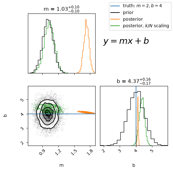
fig = corner.corner(
    walker_scaled.model_sampler.chain,
    color="tab:green",
    truths=[true_params["m"], true_params["b"]],
    labels=["m", "b"],
    show_titles=True,
)

_ = corner.corner(
    walker.model_sampler.chain,
    color="tab:orange",
    fig=fig,
)
_ = corner.corner(
    prior_distribution.rvs(10000),
    fig=fig,
)
plt.plot([], [], color="tab:blue", label="truth: $m=2, b=4$")
plt.plot([], [], color="k", label="prior")

plt.plot([], [], color="tab:orange", label="posterior")
plt.plot([], [], color="tab:green", label="posterior, $k/N$ scaling")
fig.text(0.6, 0.75, "$y=mx+b$", fontsize=20)
fig.legend(loc="upper right")
plt.tight_layout()
def predictive_posterior(
    walker, model, x, x_data, y_exp, y_err, percentile_bounds, added_noise=0.0
):
    n_posterior_samples = walker.model_sampler.chain.shape[0]
    y = np.zeros((n_posterior_samples, len(x)))
    for i in range(n_posterior_samples):
        sample = walker.model_sampler.chain[i, :]
        y[i, :] = np.random.normal(loc=model.y(x, *sample), scale=added_noise)

    percentiles = np.percentile(y, percentile_bounds, axis=0)
    return percentiles
Empirical coverage#
spacing = 10
inner_pctls = np.arange(spacing, 100, spacing)
inner_pctls
array([10, 20, 30, 40, 50, 60, 70, 80, 90])
pb = np.hstack([50 - np.flip(inner_pctls) / 2, 50 + inner_pctls / 2])
pb
array([ 5., 10., 15., 20., 25., 30., 35., 40., 45., 55., 60., 65., 70.,
       75., 80., 85., 90., 95.])
lower_bounds = np.flip(pb[: inner_pctls.shape[0]])
upper_bounds = pb[inner_pctls.shape[0] :]
for l, u in zip(lower_bounds, upper_bounds):
    print(l, u)
45.0 55.0
40.0 60.0
35.0 65.0
30.0 70.0
25.0 75.0
20.0 80.0
15.0 85.0
10.0 90.0
5.0 95.0
pctls_scaled = predictive_posterior(
    walker_scaled,
    my_model,
    x_data,
    x_data,
    y_data,
    noise,
    percentile_bounds=pb,
    added_noise=reported_stat_err,
)
pctls = predictive_posterior(
    walker,
    my_model,
    x_data,
    x_data,
    y_data,
    noise,
    percentile_bounds=pb,
    added_noise=reported_stat_err,
)
pctls_unbroadened = predictive_posterior(
    walker,
    my_model,
    x_data,
    x_data,
    y_data,
    noise,
    percentile_bounds=pb,
    added_noise=0,
)
lower = np.flip(pctls[: inner_pctls.shape[0], :], axis=0)
upper = pctls[inner_pctls.shape[0] :, :]
lower_l = np.flip(pctls_unbroadened[: inner_pctls.shape[0], :], axis=0)
upper_l = pctls_unbroadened[inner_pctls.shape[0] :, :]
lower_s = np.flip(pctls_scaled[: inner_pctls.shape[0], :], axis=0)
upper_s = pctls_scaled[inner_pctls.shape[0] :, :]
# plt.fill_between(x_data, lower_bounds[-2,:], upper_bounds[-2,:], alpha=0.5)
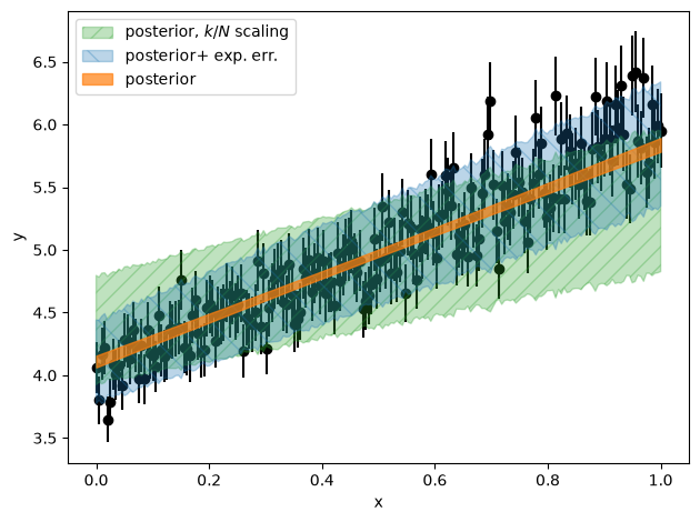
plt.errorbar(
    x_data, y_data, reported_stat_err, linestyle="none", marker="o", color="k", zorder=0
)
plt.fill_between(
    x_data,
    lower_s[-1, :],
    upper_s[-1, :],
    alpha=0.3,
    color="tab:green",
    label="posterior, $k/N$ scaling",
    hatch="//",
)

plt.fill_between(
    x_data,
    lower[-1, :],
    upper[-1, :],
    alpha=0.3,
    color="tab:blue",
    label="posterior+ exp. err.",
    hatch="\\",
)
plt.fill_between(
    x_data,
    lower_l[-1, :],
    upper_l[-1, :],
    alpha=0.7,
    color="tab:orange",
    label="posterior",
)

plt.xlabel("x")
plt.ylabel("y")
plt.legend()
plt.tight_layout()
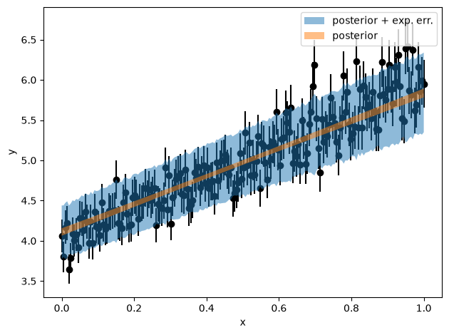
# plt.fill_between(x_data, lower_bounds[-2,:], upper_bounds[-2,:], alpha=0.5)
plt.errorbar(
    x_data, y_data, reported_stat_err, linestyle="none", marker="o", color="k", zorder=0
)
plt.fill_between(
    x_data, lower[-1, :], upper[-1, :], alpha=0.5, label="posterior + exp. err."
)
plt.fill_between(x_data, lower_l[-1, :], upper_l[-1, :], alpha=0.5, label="posterior")

plt.xlabel("x")
plt.ylabel("y")
plt.legend()
plt.tight_layout()
def coverage_counted(y, err, lower, upper):
    coverage_integrated = np.zeros(len(lower))
    for i, (l, u) in enumerate(zip(lower, upper)):
        coverage_integrated[i] = np.mean(np.logical_and(y >= l, y < u))
    return coverage_integrated
def coverage(y, err, lower, upper):
    coverage_integrated = np.zeros(len(lower))
    for i, (l, u) in enumerate(zip(lower, upper)):
        coverage_integrated[i] = np.mean(
            norm.cdf((u - y) / err) - norm.cdf((l - y) / err)
        )
    return coverage_integrated
# plt.plot(inner_pctls, coverage_sum * 100, label="sum")


# cov = coverage_counted(y_data, reported_stat_err, lower_bounds, upper_bounds)
cov = coverage_counted(y_data, reported_stat_err, lower, upper)

plt.plot(
    inner_pctls,
    cov * 100,
    label="posterior + exp. err.",
)

cov = coverage_counted(y_data, reported_stat_err, lower_l, upper_l)
# cov = coverage_counted(y_data, reported_stat_err, lower_bounds, upper_bounds)

plt.plot(
    inner_pctls,
    cov * 100,
    label="posterior",
)

plt.plot(inner_pctls, inner_pctls, "k--", label="expected")
plt.legend()
plt.xlabel("inner %")
plt.ylabel("coverage %")
plt.title(f"$N = {N}$")
plt.tight_layout()