Calibration of a line#
Simple demo demonstrating the workflow of rxmc.
from collections import OrderedDict

import corner
import numpy as np
from matplotlib import pyplot as plt
from scipy import stats

import rxmc
rng = np.random.default_rng(49)
define parameters#
help(rxmc.params.Parameter)
Help on class Parameter in module rxmc.params:

class Parameter(builtins.object)
 |  Parameter(
 |      name,
 |      dtype=<class 'float'>,
 |      unit='',
 |      latex_name=None,
 |      bounds=(-inf, inf)
 |  )
 |
 |  Methods defined here:
 |
 |  __eq__(self, other)
 |      Return self==value.
 |
 |  __init__(
 |      self,
 |      name,
 |      dtype=<class 'float'>,
 |      unit='',
 |      latex_name=None,
 |      bounds=(-inf, inf)
 |  )
 |      Parameters:
 |          name (str): Name of the parameter
 |          dtype (np.dtype): Data type of the parameter
 |          unit (str): Unit of the parameter
 |          latex_name (str): LaTeX representation of the parameter
 |          bounds (tuple, optional): Bounds for the parameter as a tuple (min, max)
 |
 |  ----------------------------------------------------------------------
 |  Data descriptors defined here:
 |
 |  __dict__
 |      dictionary for instance variables
 |
 |  __weakref__
 |      list of weak references to the object
 |
 |  ----------------------------------------------------------------------
 |  Data and other attributes defined here:
 |
 |  __hash__ = None
make the model#
help(rxmc.physical_model.PhysicalModel)
Help on class PhysicalModel in module rxmc.physical_model:

class PhysicalModel(builtins.object)
 |  PhysicalModel(params: list[rxmc.params.Parameter])
 |
 |  Represents an arbitrary parameteric model $y_{model}(x;params)$, for
 |  comparison to some experimental measurement $\{x_i, y(x_i)\}$ contained
 |  in an Observation object
 |
 |  Methods defined here:
 |
 |  __call__(self, observation: rxmc.observation.Observation, *params) -> numpy.ndarray
 |      Call self as a function.
 |
 |  __init__(self, params: list[rxmc.params.Parameter])
 |      Initialize the PhysicalModel with a list of parameters.
 |      Parameters:
 |      ----------
 |      params: list[Parameter]
 |          A list of Parameter objects that define the model's parameters.
 |          Each Parameter should have a name and a dtype.
 |
 |  evaluate(self, observation: rxmc.observation.Observation, *params) -> numpy.ndarray
 |      Evaluate the model at the given parameter values.
 |      Should be overridden by subclasses.
 |
 |      Parameters:
 |      ----------
 |      observation: Observation object containing x and y data.
 |      params: Parameters for the model, should match the model's parameters.
 |
 |  ----------------------------------------------------------------------
 |  Data descriptors defined here:
 |
 |  __dict__
 |      dictionary for instance variables
 |
 |  __weakref__
 |      list of weak references to the object
Clearly to make a model, we need to understand these things called Observations.#
This is an important detail, the whole point of rxmc is to compare predictions of a PhysicalModel to data contained in an Observation, to calibrate the parameters of the PhysicalModel.
help(rxmc.observation.Observation)
Help on class Observation in module rxmc.observation:

class Observation(builtins.object)
 |  Observation(
 |      x: numpy.ndarray,
 |      y: numpy.ndarray,
 |      y_stat_err=None,
 |      y_sys_err_normalization=None,
 |      y_sys_err_normalization_mask=None,
 |      y_sys_err_offset=None,
 |      y_sys_err_offset_mask=None
 |  )
 |
 |  A class to represent an observation with statistical errors,
 |  as well as systematic errors associated with a common normalization
 |  and offset of all or some of the data points of the the dependent
 |  variable y.
 |
 |  Attributes:
 |  ----------
 |  x : np.ndarray
 |      The independent variable data.
 |  y : np.ndarray
 |      The dependent variable data.
 |  statistical_covariance : np.ndarray
 |      The covariance matrix representing the statistical errors of y.
 |  systematic_offset_covariance : np.ndarray
 |      The covariance matrix representing systematic errors associated with
 |      the offset of y.
 |  systematic_normalization_covariance : np.ndarray
 |      The fractional covariance matrix representing systematic errors
 |      associated with the normalization of y.
 |  n_data_pts : int
 |      The number of data points in the observation.
 |
 |  Methods defined here:
 |
 |  __init__(
 |      self,
 |      x: numpy.ndarray,
 |      y: numpy.ndarray,
 |      y_stat_err=None,
 |      y_sys_err_normalization=None,
 |      y_sys_err_normalization_mask=None,
 |      y_sys_err_offset=None,
 |      y_sys_err_offset_mask=None
 |  )
 |      x : np.ndarray
 |          The independent variable data.
 |      y : np.ndarray
 |          The dependent variable data.
 |      y_stat_err : np.ndarray, optional
 |          The statistical error associated with y. Defaults to an array of
 |          zeros with the same shape as y.
 |      y_sys_err_normalization : float or array-like, optional
 |          The fractional systematic error associated with normalization of y.
 |          Defaults to 0.0.  If array-like object is passed in, that implies
 |          that there are multiple systematic errors associated with
 |          normalization, each corresponding to an entry in
 |          `y_sys_err_normalization_mask`.
 |      y_sys_err_normalization_mask : list of np.ndarray, optional
 |          Masks for the systematic errors associated with normalization of y.
 |          Each mask should have the same shape as y, and the systematic error
 |          associated with normalization will only apply to the points where
 |          the mask is True. Defaults to None, meaning no systematic errors
 |          associated with normalization, or equivalently, a single
 |          systematic error for all points.
 |      y_sys_err_offset : float or array-like, optional
 |          The systematic error associated with the offset of y. Defaults to
 |          0.0. If array-like object is passed in, that implies that there
 |          a multiple systematic errors associated with normalization, each
 |          corresponding to an entry in `y_sys_err_normalization_mask`.
 |      y_sys_err_offset_mask : list of np.ndarray, optional
 |          Masks for the systematic errors associated with the offset of y.
 |          Each mask should have the same shape as y, and the systematic error
 |          associated with the offset will only apply to the points where
 |          the mask is True. Defaults to None, meaning no systematic errors
 |          associated with the offset, or equivalently, a single systematic
 |          error for all points.
 |
 |  covariance(self, y)
 |      Returns the default covariance matrix for the observation,
 |      which is the sum of the statistical and systematic offset covariance
 |      matrices, and the fractional normalization covariance matrix
 |      multiplied by the outer product of y with itself.
 |
 |      Parameters
 |      ----------
 |      y : np.ndarray
 |          The dependent variable data for which to compute the covariance.
 |
 |  num_pts_within_interval(
 |      self,
 |      ylow: numpy.ndarray,
 |      yhigh: numpy.ndarray,
 |      xlim=None
 |  )
 |      Returns the number of points in y that fall between ylow and yhigh,
 |      useful for calculating emperical coverages
 |
 |      Parameters
 |      ----------
 |      ylow : np.ndarray, same shape as self.y
 |      yhigh : np.ndarray, same shape as self.y
 |      xlim : tuple, optional
 |          If provided, only consider points where self.x is within
 |          this range. Defaults to None, meaning all points are
 |          considered.
 |
 |      Returns
 |      -------
 |      int
 |          The number of points in self.y (within xlim) that fall
 |          within the specified interval defined by ylow and yhigh.
 |
 |  residual(self, ym: numpy.ndarray)
 |
 |  ----------------------------------------------------------------------
 |  Data descriptors defined here:
 |
 |  __dict__
 |      dictionary for instance variables
 |
 |  __weakref__
 |      list of weak references to the object
Ok, so basically it’s just some x and y, ans some information about the errors of y. We can think of Observations like experimental measurements of an observable, and we want to build a model to make uncertainty-quantified predictions of that observable.
class LinearModel(rxmc.physical_model.PhysicalModel):
    def __init__(self):
        params = [
            rxmc.params.Parameter("m", float, "no-units"),
            rxmc.params.Parameter("b", float, "y-units"),
        ]
        super().__init__(params)

    def evaluate(self, observation, m, b):
        return self.y(observation.x, m, b)

    def y(self, x, m, b):
        # useful to have a function hat takes in an array-like x
        # rather than an Observation, e.g. for plotting
        return m * x + b
Well that’s not too complicated.
my_model = LinearModel()
Let’s test it out:
# true params are obviously m = 1, b = 0
observation = rxmc.observation.Observation(x=np.array([1, 2, 3]), y=np.array([1, 2, 3]))
my_model(observation, 1, 0)
array([1, 2, 3])
my_model.y(observation.x, 2, 1)
array([3, 5, 7])
# now with parameters that are obviously wrong
my_model(observation, 2, 1)
array([3, 5, 7])
# just to show some ways that may be convenient to pass around params
# note they must be in the same order as in my_model.evaluate,
# which should be in the same order as my_model.params

p = [2, 1]
print(my_model(observation, *p))
p = np.array([2, 1])
print(my_model(observation, *p))
[3 5 7]
[3 5 7]
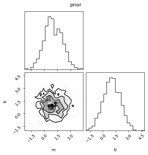
define a prior#
Let’s imagine this line corresponds to some physics, and we have some backround knowledge to inform us what we expect $m$ and $b$ to be. We can encode that into a prior distribution:
prior_mean = OrderedDict(
    [
        ("m", 1),
        ("b", 1),
    ]
)
prior_std_dev = OrderedDict(
    [
        ("m", 1),
        ("b", 1),
    ]
)
covariance = np.diag(list(prior_std_dev.values())) ** 2
mean = np.array(list(prior_mean.values()))
n_prior_samples = 1000
prior_distribution = stats.multivariate_normal(mean, covariance)
prior_samples = prior_distribution.rvs(size=n_prior_samples, random_state=rng)
Let’s plot some samples of lines from this prior
x = np.linspace(0, 1, 10)

# array to hold the lines
y = np.zeros((n_prior_samples, len(x)))

# propagate the prior through to the observation
for i in range(n_prior_samples):
    sample = prior_samples[i, :]
    y[i, :] = my_model.y(x, *sample)

# grab confidence intervals for plotting
upper, lower = np.percentile(y, [5, 95], axis=0)
for i in np.random.choice(n_prior_samples, 1000):
    plt.plot(x, y[i, :], zorder=1, alpha=0.2)
    # pass

plt.fill_between(
    x, lower, upper, alpha=0.5, zorder=2, label=r"inner 90$^\text{th}$ pctl"
)
plt.xlabel("x")
plt.ylabel("y")
plt.legend()
plt.title("prior")
Text(0.5, 1.0, 'prior')
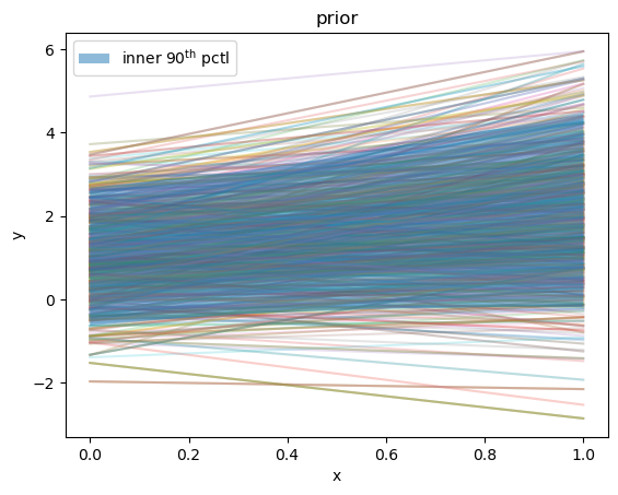
fig = corner.corner(prior_samples, labels=[p.name for p in my_model.params])
fig.suptitle("prior")
Text(0.5, 0.98, 'prior')
Now let’s update our prior by comparing to some data#
This will require learning about LikelihoodModels in rxmc. These encode our assumptions about the error on an experimental Observation, and are a necessary ingredient for comparing to the predictions of a PhysicalModel.
In our case we will mock experimental data by synthetically generate some data with noise about a “true” $m$ and $b$. Our calibration posterior should converge to be centered about this true point.
Let us assume that the experimentalists made a perfect estimate of the experimental noise in their setup. That is, the error bars they report will correspond exactly to the true distribution from which we sample.
This noise will correspond to statistical noise. Later on we will look at systematic experimental error.
true_params = OrderedDict(
    [
        ("m", 0.6),
        ("b", 2),
    ]
)

x = np.linspace(0, 1, 10)
noise = 0.1
y_exp = my_model.y(x, *list(true_params.values())) + rng.normal(
    scale=noise, size=len(x)
)
y_stat_err = noise * np.ones_like(y_exp)  # noise is just a constant fraction of y
obs1 = rxmc.observation.Observation(x=x, y=y_exp, y_stat_err=y_stat_err)
plt.errorbar(
    x,
    y_exp,
    y_stat_err,
    color="k",
    marker=".",
    linestyle="none",
    label="obs1",
)
plt.plot(x, my_model.y(x, *list(true_params.values())), "k--", label="truth")
plt.xlabel("x")
plt.ylabel("y")

plt.fill_between(
    x,
    lower,
    upper,
    alpha=0.5,
    zorder=2,
    label=r"prior inner 90$^\text{th}$ pctl",
)

plt.legend()
plt.title("experimental constraint")
Text(0.5, 1.0, 'experimental constraint')
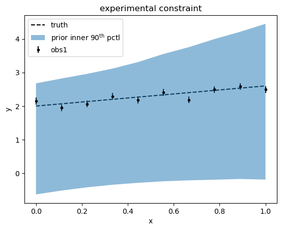
Clearly, our prior is at odds with our observation. We will now determine a posterior distribution of $m$ and $b$ that takes obs1 into account. To do this, we will need to think about a LikelihoodModel for obs1.
set up LikelihoodModel and Constraint.#
We will use the simplest assumption about the error on y: that the experimentalists exactly reported the statistical error, and there is no systematic error at all. This implies that each data point in obs1.y, say obs1.y[i] can be modeled as being an random variate, each sampled independently from normal distributions with mean obs1.y[i] and with standard deviation obs1.y_stat_err[i].
This behavior is handled by the default LikelihoodModel:
help(rxmc.likelihood_model.LikelihoodModel)
Help on class LikelihoodModel in module rxmc.likelihood_model:

class LikelihoodModel(builtins.object)
 |  A class to represent a likelihood model for comparing an Observation
 |  to a PhysicalModel.
 |
 |  The default behavior uses the following covariance matrix:
 |      \[
 |          \Sigma_{ij} = \sigma^2_{i}^{stat} \delta_{ij}
 |                      + \Sigma_{ij}^{sys}
 |                      + \gamma^2 y_m^2(x_i, \alpha)
 |      \]
 |  where $sigma^2_{i}^{stat}$ is the statistical variance of the i-th
 |  observation, (`observation.statistical_covariance`) and $\gamma$ is the
 |  fractional uncorrelated error (`self.frac_err`).
 |
 |  Here, $Sigma_{ij}^{sys}$ is the systematic covariance matrix:
 |      \[
 |          \Sigma_{ij}^{sys} = \eta**2 y_m(x_i, \alpha) y_m(x_j, \alpha) + \omega,
 |      \]
 |  where $\eta$ is the uncertainty in the overall normalization of the
 |  observation (`observation.y_sys_err_normalization`) and $\omega$ is the
 |  uncertainty in the additive normalization to the observation
 |  (`observation.y_sys_err_offset`).
 |
 |  Here, also, $y_m(x_i, \alpha)$ is the model prediction for the i-th
 |  observation. Thus the covariance matrix is dependent on the values
 |  of the PhysicalModel and its parameters, as is the case when systematic
 |  errors are present in the observation, following D'Agostini, G. (1993) 'On
 |  the use of the covariance matrix to fit correlated data'
 |
 |  Note that if there is no systematic uncertainty encoded in the `observation`
 |  and `self.frac_err` takes the default value of 0, the
 |  covariance matrix becomes diaginal, and the `chi2` function reduces to the
 |  simple and familiar $\chi^2$ form.
 |
 |  Note also that this is equivalent to the alternative method to handle systematic
 |  errors described by Barlow, R (2021) 'Combining experiments with systematic
 |  errors', in which nuisance parameters are introduced corresponding to the
 |  normalization and additive offset bias of the observation.
 |
 |  The advantage of this approach is that it does not require introducing
 |  nuisance parameters, but instead encodes the correlation between the data
 |  points in the observation in the covariance matrix directly.
 |
 |  Methods defined here:
 |
 |  __init__(self)
 |      Initializes the LikelihoodModel, optionally with a fractional
 |      uncorrelated error.
 |
 |  chi2(self, observation: rxmc.observation.Observation, ym: numpy.ndarray)
 |      Calculate the generalised chi-squared statistic. This is the
 |      square of the Mahalanobis distance between y and ym
 |
 |      Parameters
 |      ----------
 |      observation : Observation
 |          The observation object containing the observed data.
 |      ym : np.ndarray
 |          Model prediction for the observation.
 |
 |      Returns
 |      -------
 |      float
 |          Chi-squared statistic.
 |
 |  covariance(self, observation: rxmc.observation.Observation, ym: numpy.ndarray)
 |      Default covariance model. Derived classes of `LikelihoodModel` will
 |      override this.
 |
 |      Returns the following covariance matrix:
 |          \[
 |              \Sigma_{ij} = \sigma^2_{i}^{stat} \delta_{ij}
 |                          + \Sigma_{ij}^{sys}
 |                          + \gamma^2 y_m^2(x_i, \alpha)
 |          \]
 |      where $sigma^2_{i}^{stat}$ is the statistical variance of the i-th
 |      observation, (`observation.statistical_covariance`) and $\gamma$ is the
 |      fractional uncorrelated error (`self.frac_err`).
 |
 |      Here, $Sigma_{ij}^{sys}$ is the systematic covariance matrix:
 |          \[
 |              \Sigma_{ij}^{sys} = \eta**2 y_m(x_i, \alpha) y_m(x_j, \alpha) + \omega,
 |          \]
 |      where $\eta$ is the uncertainty in the overall normalization of the
 |      observation (`observation.y_sys_err_normalization`) and $\omega$ is the
 |      uncertainty in the additive normalization to the observation
 |      (`observation.y_sys_err_offset`).
 |
 |      Here, also, $y_m(x_i, \alpha)$ is the model prediction for the i-th
 |      observation.
 |
 |      Parameters
 |      ----------
 |      ym : np.ndarray
 |          Model prediction for the observation.
 |      observation : Observation
 |          The observation object containing the observed data.
 |
 |      Returns
 |      -------
 |      np.ndarray
 |          Covariance matrix of the observation.
 |
 |  log_likelihood(
 |      self,
 |      observation: rxmc.observation.Observation,
 |      ym: numpy.ndarray
 |  )
 |      Returns the log_likelihood that ym reproduces y, given the covariance
 |
 |      Parameters
 |      ----------
 |      ym : np.ndarray
 |          Model prediction for the observation.
 |      observation : Observation
 |          The observation object containing the observed data.
 |
 |      Returns
 |      -------
 |      float
 |
 |  residual(self, observation: rxmc.observation.Observation, ym: numpy.ndarray)
 |      Returns the residual between the model prediction ym and
 |      observation.y
 |
 |      Parameters:
 |      ----------
 |      observation : Observation
 |          The observation object containing the observed data.
 |      ym : np.ndarray
 |          Model prediction for the observation.
 |
 |      Returns
 |      -------
 |      np.ndarray
 |          Residual vector.
 |
 |  ----------------------------------------------------------------------
 |  Data descriptors defined here:
 |
 |  __dict__
 |      dictionary for instance variables
 |
 |  __weakref__
 |      list of weak references to the object
Sorry, I know that’s a lot to read. The important piece is right here:
| Note that if there is no systematic uncertainty encoded in the observation
| and self.fractional_uncorrelated_error takes the default value of 0, the
| covariance matrix becomes diaginal, and the chi2 function reduces to the
| simple and familiar $\chi^2$ form.
This means that, in our case in which the errors are only statistical, the likelihood will be porportional to the familiar form:
\begin{equation} \mathcal{L}(\alpha|y) \propto e^{ - \chi^2(\alpha,y) } \end{equation}
where the Chi-squared is simply
\begin{equation} \chi^2(\alpha,y) = \sum_i \frac{(y(x_i) - y_m(x_i;\alpha) )^2}{\sigma^2_i} \end{equation}
In a later tutorial we will use more complicated Observations that include systematic error, and look at other LikelihoodModels.
likelihood_model = rxmc.likelihood_model.LikelihoodModel()
constraint = rxmc.constraint.Constraint(
    [obs1],
    my_model,
    likelihood_model,
)
Let’s test this constraint thing out. What is the reduced $\chi^2$ for the prior mean?
constraint.chi2(prior_distribution.mean) / constraint.n_data_pts
np.float64(64.18631209285807)
Here is proof that, in this case, we reduce to the form described above:
y = my_model(obs1, *prior_distribution.mean)
np.sum((y - obs1.y) ** 2 / y_stat_err**2) / constraint.n_data_pts
np.float64(64.18631209285807)
running the calibration#
help(rxmc.walker.Walker)
Help on class Walker in module rxmc.walker:

class Walker(builtins.object)
 |  Walker(
 |      model_sampler: rxmc.param_sampling.Sampler,
 |      evidence: rxmc.evidence.Evidence,
 |      likelihood_samplers: list[rxmc.param_sampling.Sampler] = [],
 |      rng: numpy.random._generator.Generator = Generator(PCG64) at 0x14FA84891460
 |  )
 |
 |  A class that encapsulates the sampling configuration for a Bayesian
 |  inference problem, including the physical model and likelihood model
 |  configurations. It manages the sampling process for both the physical
 |  model and the likelihood model parameters, alternating between each
 |  model in a Gibbs sampling framework.
 |
 |  Methods defined here:
 |
 |  __init__(
 |      self,
 |      model_sampler: rxmc.param_sampling.Sampler,
 |      evidence: rxmc.evidence.Evidence,
 |      likelihood_samplers: list[rxmc.param_sampling.Sampler] = [],
 |      rng: numpy.random._generator.Generator = Generator(PCG64) at 0x14FA84891460
 |  )
 |      Initialize the Sampler with a list of samplers.
 |
 |      Parameters:
 |      ----------
 |      model_sampler: Sampler
 |          A Sampler object for physical model parameters.
 |      evidence: Evidence
 |          A Evidence object containing the data for which the likelihood
 |          model is evaluated.
 |      likelihood_model_samplers: list[Sampler]
 |          A list of Sampler objects for likelihood model parameters.
 |          Corresponds to the order of `evidence.parametric_constraints`.
 |      rng: np.random.Generator, optional
 |          A random number generator for reproducibility. Defaults to a new
 |          default_rng with a fixed seed.
 |
 |  log_likelihood(self, model_params, likelihood_params)
 |
 |  log_posterior(self, model_params, likelihood_params)
 |
 |  log_prior(self, model_params, likelihood_params)
 |      Returns the log-prior probability of the model parameters and
 |      likelihood parameters.
 |
 |      Parameters:
 |      ----------
 |      model_params: tuple
 |          The parameters of the physical model.
 |      likelihood_params: list[tuple]
 |          A list of tuples containing additional parameters for the
 |          likelihood model for each constraint.
 |
 |      Returns:
 |      -------
 |      float
 |          The log-prior probability.
 |
 |  run_likelihood_batches(
 |      self,
 |      n_steps,
 |      starting_locations,
 |      model_params,
 |      burn=False
 |  )
 |      Walks each of the likelihood parameter spacers one by one, for a
 |      fixed value of `model_params`
 |
 |      Parameters:
 |      ----------
 |      n_steps: int
 |          The number of steps to run for each likelihood model.
 |      starting_locations: list[np.ndarray]
 |          A list of starting locations for each likelihood model.
 |      model_params: tuple
 |          A fixed value of the parameters for the physical model
 |      burn: bool
 |          If True, the batch is considered a burn-in batch and
 |          the acceptance rate, log probabilities, and parameter
 |          chain will not be recorded.
 |
 |      Returns:
 |      -------
 |      list[np.ndarray]
 |          A list of parameter chains for each likelihood model.
 |      logp : list[np.ndarray]
 |          A list of log probabilities for each likelihood model.
 |      accepted : list[float]
 |          A list of acceptance rates for each likelihood model.
 |
 |  run_model_batch(self, n_steps, x0, likelihood_params=[], burn=False)
 |      Walks the model parameter space for fixed values of the
 |      `likelihood_params`
 |
 |      Parameters:
 |      ----------
 |      n_steps: int
 |          The number of steps to run for the model sampling.
 |      x0: np.ndarray
 |          The starting location for the model sampling.
 |      likelihood_params: list[tuple]
 |          A list of fixed values of the parameters for each of the
 |          parametric likelihood models, corresponding to the order
 |          of `self.likelihood_samplers`
 |      burn: bool
 |          If True, the batch is considered a burn-in batch and
 |          the acceptance rate, log probabilities, and parameter
 |          chain will not be recorded.
 |
 |      Returns:
 |      -------
 |      batch_chain: np.ndarray
 |          The parameter chain generated by the model sampling algorithm.
 |      logp: np.ndarray
 |          The log probabilities of the parameter chain.
 |      accepted: float
 |          The acceptance rate of the model sampling algorithm.
 |
 |  walk(
 |      self,
 |      n_steps: int,
 |      burnin: int = 0,
 |      batch_size: int = None,
 |      verbose: bool = True
 |  )
 |      Runs the MCMC chain with the specified parameters.
 |      Updates the internal state of the `model_sampler` and
 |      `likelihood_samplers` with records of the walk and relevant
 |      statistics.
 |
 |      Parameters:
 |      -----------
 |          n_steps : int
 |              Total number of active steps for the MCMC chain.
 |          batch_size : int
 |              Number of steps per batch.
 |          burnin : int
 |              Number of extra burn-in steps to do before active steps
 |          verbose : bool
 |              Flag to print extra logging information.
 |
 |  ----------------------------------------------------------------------
 |  Data descriptors defined here:
 |
 |  __dict__
 |      dictionary for instance variables
 |
 |  __weakref__
 |      list of weak references to the object
First we need to put together our Evidence. With one constraint this seems trivial, but this will be useful down the road when we may want to combine multiple constraints together.
evidence = rxmc.evidence.Evidence([constraint])
Another chore we have to do is configure how we will sample our parameter space.
help(rxmc.param_sampling.MetropolisHastingsSampler)
Help on class MetropolisHastingsSampler in module rxmc.param_sampling:

class MetropolisHastingsSampler(Sampler)
 |  MetropolisHastingsSampler(
 |      params: list[rxmc.params.Parameter],
 |      prior,
 |      starting_location: numpy.ndarray,
 |      proposal: rxmc.proposal.ProposalDistribution
 |  )
 |
 |  Metropolis-Hastings sampler. The ol' reliable.
 |
 |  Method resolution order:
 |      MetropolisHastingsSampler
 |      Sampler
 |      builtins.object
 |
 |  Methods defined here:
 |
 |  __init__(
 |      self,
 |      params: list[rxmc.params.Parameter],
 |      prior,
 |      starting_location: numpy.ndarray,
 |      proposal: rxmc.proposal.ProposalDistribution
 |  )
 |      Parameters:
 |      ----------
 |      params: list[params.Parameter]
 |          List of parameters to sample.
 |      prior: object
 |          Prior distribution object that has a method `logpdf`.
 |      starting_location: np.ndarray
 |          Initial parameter values for the chain.
 |      proposal: proposal.ProposalDistribution
 |          Proposal distribution object that has a method `__call__` which
 |          takes in a parameter vector and an rng, returning a proposed
 |          parameter vector.
 |
 |  ----------------------------------------------------------------------
 |  Methods inherited from Sampler:
 |
 |  batch_acceptance_fractions(self) -> numpy.ndarray
 |      Returns the acceptance fraction of the sampler in each batch run.
 |
 |  most_recent_batch_acceptance_fraction(self) -> float
 |      Returns the acceptance fraction of the most recent batch run.
 |
 |  overall_acceptance_fraction(self) -> float
 |      Returns the overall acceptance fraction of the sampler.
 |
 |  record_batch(
 |      self,
 |      n_steps: int,
 |      n_accepted: int,
 |      chain: numpy.ndarray,
 |      logp_chain: numpy.ndarray
 |  )
 |      Records the batch of samples and acceptance statistics.
 |
 |      Parameters:
 |      ----------
 |      n_steps: int
 |          Number of steps in the batch.
 |      n_accepted: int
 |          Number of accepted samples in the batch.
 |      chain: np.ndarray
 |          Array of sampled parameter vectors.
 |      logp_chain: np.ndarray
 |          Array of log posterior values corresponding to the sampled parameter vectors.
 |
 |  sample(
 |      self,
 |      n_steps: int,
 |      starting_location: numpy.ndarray,
 |      rng: numpy.random._generator.Generator,
 |      log_posterior: Callable[[numpy.ndarray], float],
 |      burn: bool = False
 |  )
 |      Samples from the posterior distribution using the specified
 |      sampling algorithm, updating the state and recording the chain,
 |      log posterior values, and acceptance statistics.
 |
 |      Parameters:
 |      ----------
 |      n_steps: int
 |          Number of steps to sample.
 |      starting_location: np.ndarray
 |          Initial parameter values for the chain.
 |      rng: np.random.Generator
 |          Random number generator for reproducibility.
 |      log_posterior: Callable[[np.ndarray], float]
 |          Function that computes the log posterior probability of
 |          a parameter vector.
 |      burn: bool
 |          If True, the samples are considered burn-in and will not
 |          be recorded in the chain, only the current state will be updated.
 |
 |  ----------------------------------------------------------------------
 |  Data descriptors inherited from Sampler:
 |
 |  __dict__
 |      dictionary for instance variables
 |
 |  __weakref__
 |      list of weak references to the object
This means we have to decide on a proposal distribution. We will use a simple form: just sampling from a scaled down version of the prior about the previos point:
def proposal_distribution(x, rng):
    return stats.multivariate_normal.rvs(
        mean=x, cov=prior_distribution.cov / 100, random_state=rng
    )
sampling_config = rxmc.param_sampling.MetropolisHastingsSampler(
    params=my_model.params,
    starting_location=prior_distribution.mean,
    proposal=proposal_distribution,
    prior=prior_distribution,
)
walker = rxmc.walker.Walker(
    sampling_config,
    evidence,
)
%%time
walker.walk(
    n_steps=20000,
    burnin=1000,
)
Burn-in batch 1/1 completed, 1000 steps.
Batch: 1/1 completed, 20000 steps.
  Model parameter acceptance fraction: 0.273
CPU times: user 6.51 s, sys: 151 ms, total: 6.66 s
Wall time: 7.97 s
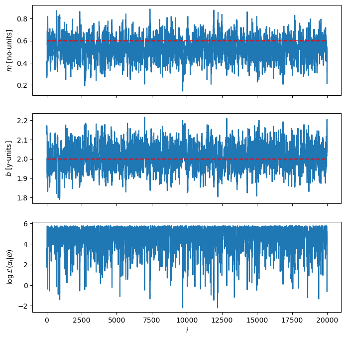
chain = walker.model_sampler.chain
logp = walker.model_sampler.logp_chain
chain.shape
(20000, 2)
fig, axes = plt.subplots(chain.shape[1] + 1, 1, figsize=(8, 8), sharex=True)
for i in range(chain.shape[1]):
    axes[i].plot(chain[:, i])
    axes[i].set_ylabel(f"${my_model.params[i].latex_name}$ [{my_model.params[i].unit}]")
    true_value = true_params[my_model.params[i].name]
    axes[i].hlines(true_value, 0, len(chain), "r", linestyle="--")


axes[-1].plot(logp)
axes[-1].set_ylabel(r"$\log{\mathcal{L}(\alpha_i | \mathcal{O})}$")

axes[-1].set_xlabel(r"$i$")
# plt.legend(title="chains", ncol=3,)
Text(0.5, 0, '$i$')
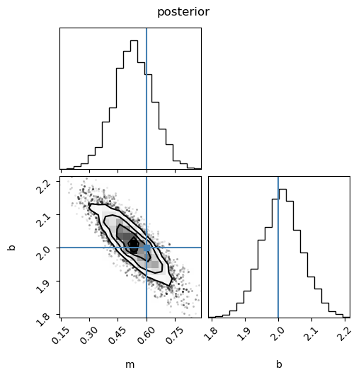
posterior_range = np.vstack([np.min(chain, axis=0), np.max(chain, axis=0)]).T
fig = corner.corner(
    chain,
    labels=[p.name for p in my_model.params],
    label="posterior",
    truths=[true_params["m"], true_params["b"]],
)
fig.suptitle("posterior")
Text(0.5, 0.98, 'posterior')
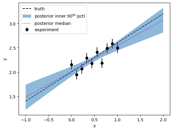
x_full = np.linspace(-1, 2, 10)
n_posterior_samples = chain.shape[0]
y = np.zeros((n_posterior_samples, len(x_full)))
for i in range(n_posterior_samples):
    sample = chain[i, :]
    y[i, :] = my_model.y(x_full, *sample)

upper, median, lower = np.percentile(y, [5, 50, 95], axis=0)
plt.plot(x_full, my_model.y(x_full, *list(true_params.values())), "k--", label="truth")
plt.xlabel("x")
plt.ylabel("y")
plt.errorbar(
    x,
    obs1.y,
    y_stat_err,
    color="k",
    marker="o",
    linestyle="none",
    label="experiment",
)
plt.fill_between(
    x_full,
    lower,
    upper,
    alpha=0.5,
    zorder=2,
    label=r"posterior inner 90$^\text{th}$ pctl",
)
plt.plot(x_full, median, "m:", label="posterior median")

plt.legend()
# plt.title("predictive posterior")
<matplotlib.legend.Legend at 0x14fa68dad1d0>
Nice!#
Hopefully this simple example served to illustrate the basic function of the working pieces of rxmc. The true power is the ability to compose different Constraints, and easily manage and test different model forms for both the PhysicalModel and LikelihoodModel.
Check out the other demos to see how rxmc helps us handle more realistic problems.