Bayesian calibration of polynomials, including inference of overall normalization

import corner

import numpy as np
from matplotlib import pyplot as plt
from scipy import stats

import rxmc

Using database version X4-2025-12-31 located in: /mnt/home/beyerkyl/x4db/unpack_exfor-2025/X4-2025-12-31

rng = np.random.default_rng(42)

poly4 = rxmc.physical_model.Polynomial(4)

true_params = [1, 0.5, -0.1, -0.4, 0.1]

settings = [
    {
        "domain": [-0.3, 0.4],
        "N": 50,
        "noise": 0.1,
        "systematic_err": 0.1,
    },
    {
        "domain": [0.3, 0.5],
        "N": 30,
        "noise": 0.1,
        "systematic_err": 0.5,
    },
    {
        "domain": [0.1, 0.6],
        "N": 25,
        "noise": 0.1,
        "systematic_err": 0.2,
    },
    {
        "domain": [-0.5, 0.1],
        "N": 15,
        "noise": 0.2,
        "systematic_err": 0.6,
    },
]

def generate_observations(settings, true_model, rng, true_params, scale_err=True):
    obs = []
    for setting in settings:
        x0, x1 = setting["domain"]
        synthetic_obs = rxmc.observation.Observation(
            x=rng.random(setting["N"]) * (x1 - x0) + x0,
            y=np.zeros(setting["N"]),
            y_stat_err=np.ones(setting["N"]) * setting["noise"],
            y_sys_err_normalization=setting["systematic_err"],
        )
        renormalization = rng.normal(1, setting["systematic_err"])
        y_true = true_model(synthetic_obs, *true_params)
        if scale_err:
            synthetic_obs.y = rng.normal(y_true, setting["noise"]) * renormalization
        else:
            synthetic_obs.y = rng.normal(y_true * renormalization, setting["noise"])

        synthetic_obs.renormalization = renormalization

        obs.append(synthetic_obs)
    return obs

observations = generate_observations(settings, poly4, rng, true_params, scale_err=False)

observations_unreported_sys_err = [
    rxmc.observation.Observation(
        x=obs.x,
        y=obs.y,
        y_stat_err=np.sqrt(np.diag(obs.statistical_covariance)),
    )
    for obs in observations
]

N_fine = 100
domain_fine = (-1, 1)
truth = rxmc.observation.Observation(
    x=np.linspace(*domain_fine, N_fine), y=np.zeros(N_fine)
)
truth.y = poly4(truth, *true_params)

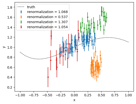
plt.plot(truth.x, truth.y, "k:", label="truth")
for synthetic_observation in observations:
    plt.errorbar(
        synthetic_observation.x,
        synthetic_observation.y,
        np.sqrt(np.diag(synthetic_observation.statistical_covariance)),
        linestyle="none",
        marker=".",
        label=f"renormalization = {synthetic_observation.renormalization:1.3f}",
    )
plt.xlabel("x")
plt.ylabel("y")
plt.legend()

<matplotlib.legend.Legend at 0x14a5192e4590>

correct_model = poly4

evidence_models = {}
evidence_models["unknown_norm"] = rxmc.evidence.Evidence(
    parametric_constraints=[
        rxmc.constraint.Constraint(
            [obs],
            correct_model,
            rxmc.likelihood_model.UnknownNormalizationModel(),
        )
        for obs in observations
    ]
)

evidence_models["marginalized_sys_err"] = rxmc.evidence.Evidence(
    [
        rxmc.constraint.Constraint(
            observations,
            correct_model,
            rxmc.likelihood_model.LikelihoodModel(),
        )
    ]
)
evidence_models["unreported_sys_err"] = rxmc.evidence.Evidence(
    [
        rxmc.constraint.Constraint(
            observations_unreported_sys_err,
            correct_model,
            rxmc.likelihood_model.LikelihoodModel(),
        )
    ]
)

evidence_models["unreported_sys_err_with_unknown_model_err"] = rxmc.evidence.Evidence(
    parametric_constraints=[
        rxmc.constraint.Constraint(
            observations_unreported_sys_err,
            correct_model,
            rxmc.likelihood_model.UnknownModelError(),
        )
    ]
)

evidence_models.keys()

dict_keys(['unknown_norm', 'marginalized_sys_err', 'unreported_sys_err', 'unreported_sys_err_with_unknown_model_err'])

print("hyperparameters for each model:")
hyperparams = {}
for key, evidence_model in evidence_models.items():
    hyperparams[key] = []
    for constraint in evidence_model.parametric_constraints:
        for p in constraint.likelihood.params:
            hyperparams[key].append(p)
    print(f"{key}: {[p.name for p in hyperparams[key]]}")

hyperparameters for each model:
unknown_norm: ['log normalization', 'log normalization', 'log normalization', 'log normalization']
marginalized_sys_err: []
unreported_sys_err: []
unreported_sys_err_with_unknown_model_err: ['log fractional err']

Priors

We will put a tight prior on $a_0$, to avoid identifiability issues, as $a_0$ corresponds to an additive offset of the entire model, which is pretty confounding with a multiplicative bias.

cov = np.diag(np.ones(len(correct_model.params)))
cov[0, 0] = 0.001
model_prior = stats.multivariate_normal(mean=np.array([1, 0, 0, 0, 0]), cov=cov)

unknown_log_norm_priors = [
    stats.multivariate_normal(
        mean=[0], cov=[[np.log(1 + (setting["systematic_err"]) ** 2)]]
    )
    for setting in settings
]

unknown_model_err_prior = stats.multivariate_normal(mean=[np.log(0.1)], cov=[[0.01]])

Walkers

walkers = {}

walkers["unknown_norm"] = rxmc.walker.Walker(
    model_sampler=rxmc.param_sampling.BatchedAdaptiveMetropolisSampler(
        correct_model.params,
        starting_location=model_prior.mean,
        prior=model_prior,
        initial_proposal_cov=model_prior.cov,
    ),
    evidence=evidence_models["unknown_norm"],
    likelihood_samplers=[
        rxmc.param_sampling.BatchedAdaptiveMetropolisSampler(
            params=[p],
            starting_location=np.array([0.0]),
            prior=prior,
            initial_proposal_cov=[[prior.cov]],
        )
        for p, prior in zip(hyperparams["unknown_norm"], unknown_log_norm_priors)
    ],
)

walkers["unreported_sys_err_with_unknown_model_err"] = rxmc.walker.Walker(
    model_sampler=rxmc.param_sampling.BatchedAdaptiveMetropolisSampler(
        correct_model.params,
        starting_location=model_prior.mean,
        prior=model_prior,
        initial_proposal_cov=model_prior.cov,
    ),
    evidence=evidence_models["unreported_sys_err_with_unknown_model_err"],
    likelihood_samplers=[
        rxmc.param_sampling.BatchedAdaptiveMetropolisSampler(
            params=hyperparams["unreported_sys_err_with_unknown_model_err"],
            starting_location=unknown_model_err_prior.mean,
            prior=unknown_model_err_prior,
            initial_proposal_cov=unknown_model_err_prior.cov,
        )
    ],
)

walkers["marginalized_sys_err"] = rxmc.walker.Walker(
    model_sampler=rxmc.param_sampling.BatchedAdaptiveMetropolisSampler(
        correct_model.params,
        starting_location=model_prior.mean,
        prior=model_prior,
        initial_proposal_cov=model_prior.cov,
    ),
    evidence=evidence_models["marginalized_sys_err"],
)

walkers["unreported_sys_err"] = rxmc.walker.Walker(
    model_sampler=rxmc.param_sampling.BatchedAdaptiveMetropolisSampler(
        correct_model.params,
        starting_location=model_prior.mean,
        prior=model_prior,
        initial_proposal_cov=model_prior.cov,
    ),
    evidence=evidence_models["unreported_sys_err"],
)

for key, walker in walkers.items():
    print(f"\nRunning {key}")
    walker.walk(n_steps=20000, burnin=8000, batch_size=2000)

Running unknown_norm
Burn-in batch 1/4 completed, 2000 steps.
Burn-in batch 2/4 completed, 2000 steps.
Burn-in batch 3/4 completed, 2000 steps.
Burn-in batch 4/4 completed, 2000 steps.
Batch: 1/10 completed, 2000 steps. 
  Model parameter acceptance fraction: 0.270
  Likelihood parameter acceptance fractions: [0.449, 0.435, 0.452, 0.455]
Batch: 2/10 completed, 2000 steps. 
  Model parameter acceptance fraction: 0.322
  Likelihood parameter acceptance fractions: [0.443, 0.4335, 0.449, 0.4255]
Batch: 3/10 completed, 2000 steps. 
  Model parameter acceptance fraction: 0.289
  Likelihood parameter acceptance fractions: [0.4415, 0.425, 0.4535, 0.4425]
Batch: 4/10 completed, 2000 steps. 
  Model parameter acceptance fraction: 0.276
  Likelihood parameter acceptance fractions: [0.4595, 0.45, 0.4375, 0.451]
Batch: 5/10 completed, 2000 steps. 
  Model parameter acceptance fraction: 0.298
  Likelihood parameter acceptance fractions: [0.45, 0.453, 0.4525, 0.442]
Batch: 6/10 completed, 2000 steps. 
  Model parameter acceptance fraction: 0.324
  Likelihood parameter acceptance fractions: [0.4385, 0.4445, 0.4165, 0.4395]
Batch: 7/10 completed, 2000 steps. 
  Model parameter acceptance fraction: 0.240
  Likelihood parameter acceptance fractions: [0.4675, 0.437, 0.445, 0.442]
Batch: 8/10 completed, 2000 steps. 
  Model parameter acceptance fraction: 0.321
  Likelihood parameter acceptance fractions: [0.431, 0.4055, 0.4555, 0.474]
Batch: 9/10 completed, 2000 steps. 
  Model parameter acceptance fraction: 0.284
  Likelihood parameter acceptance fractions: [0.4395, 0.4685, 0.4455, 0.4145]
Batch: 10/10 completed, 2000 steps. 
  Model parameter acceptance fraction: 0.290
  Likelihood parameter acceptance fractions: [0.4525, 0.441, 0.4225, 0.462]

Running unreported_sys_err_with_unknown_model_err
Burn-in batch 1/4 completed, 2000 steps.
Burn-in batch 2/4 completed, 2000 steps.
Burn-in batch 3/4 completed, 2000 steps.
Burn-in batch 4/4 completed, 2000 steps.
Batch: 1/10 completed, 2000 steps. 
  Model parameter acceptance fraction: 0.285
  Likelihood parameter acceptance fractions: [0.4255]
Batch: 2/10 completed, 2000 steps. 
  Model parameter acceptance fraction: 0.327
  Likelihood parameter acceptance fractions: [0.4595]
Batch: 3/10 completed, 2000 steps. 
  Model parameter acceptance fraction: 0.276
  Likelihood parameter acceptance fractions: [0.4475]
Batch: 4/10 completed, 2000 steps. 
  Model parameter acceptance fraction: 0.279
  Likelihood parameter acceptance fractions: [0.464]
Batch: 5/10 completed, 2000 steps. 
  Model parameter acceptance fraction: 0.293
  Likelihood parameter acceptance fractions: [0.4575]
Batch: 6/10 completed, 2000 steps. 
  Model parameter acceptance fraction: 0.295
  Likelihood parameter acceptance fractions: [0.453]
Batch: 7/10 completed, 2000 steps. 
  Model parameter acceptance fraction: 0.287
  Likelihood parameter acceptance fractions: [0.4415]
Batch: 8/10 completed, 2000 steps. 
  Model parameter acceptance fraction: 0.304
  Likelihood parameter acceptance fractions: [0.429]
Batch: 9/10 completed, 2000 steps. 
  Model parameter acceptance fraction: 0.314
  Likelihood parameter acceptance fractions: [0.432]
Batch: 10/10 completed, 2000 steps. 
  Model parameter acceptance fraction: 0.309
  Likelihood parameter acceptance fractions: [0.4585]

Running marginalized_sys_err
Burn-in batch 1/4 completed, 2000 steps.
Burn-in batch 2/4 completed, 2000 steps.
Burn-in batch 3/4 completed, 2000 steps.
Burn-in batch 4/4 completed, 2000 steps.
Batch: 1/10 completed, 2000 steps. 
  Model parameter acceptance fraction: 0.292
Batch: 2/10 completed, 2000 steps. 
  Model parameter acceptance fraction: 0.319
Batch: 3/10 completed, 2000 steps. 
  Model parameter acceptance fraction: 0.306
Batch: 4/10 completed, 2000 steps. 
  Model parameter acceptance fraction: 0.319
Batch: 5/10 completed, 2000 steps. 
  Model parameter acceptance fraction: 0.277
Batch: 6/10 completed, 2000 steps. 
  Model parameter acceptance fraction: 0.290
Batch: 7/10 completed, 2000 steps. 
  Model parameter acceptance fraction: 0.287
Batch: 8/10 completed, 2000 steps. 
  Model parameter acceptance fraction: 0.299
Batch: 9/10 completed, 2000 steps. 
  Model parameter acceptance fraction: 0.300
Batch: 10/10 completed, 2000 steps. 
  Model parameter acceptance fraction: 0.290

Running unreported_sys_err
Burn-in batch 1/4 completed, 2000 steps.
Burn-in batch 2/4 completed, 2000 steps.
Burn-in batch 3/4 completed, 2000 steps.
Burn-in batch 4/4 completed, 2000 steps.
Batch: 1/10 completed, 2000 steps. 
  Model parameter acceptance fraction: 0.275
Batch: 2/10 completed, 2000 steps. 
  Model parameter acceptance fraction: 0.288
Batch: 3/10 completed, 2000 steps. 
  Model parameter acceptance fraction: 0.299
Batch: 4/10 completed, 2000 steps. 
  Model parameter acceptance fraction: 0.286
Batch: 5/10 completed, 2000 steps. 
  Model parameter acceptance fraction: 0.294
Batch: 6/10 completed, 2000 steps. 
  Model parameter acceptance fraction: 0.331
Batch: 7/10 completed, 2000 steps. 
  Model parameter acceptance fraction: 0.286
Batch: 8/10 completed, 2000 steps. 
  Model parameter acceptance fraction: 0.296
Batch: 9/10 completed, 2000 steps. 
  Model parameter acceptance fraction: 0.289
Batch: 10/10 completed, 2000 steps. 
  Model parameter acceptance fraction: 0.293

colors = dict(
    zip(walkers.keys(), ["tab:blue", "tab:orange", "tab:purple", "tab:green"])
)
colors

{'unknown_norm': 'tab:blue',
 'unreported_sys_err_with_unknown_model_err': 'tab:orange',
 'marginalized_sys_err': 'tab:purple',
 'unreported_sys_err': 'tab:green'}

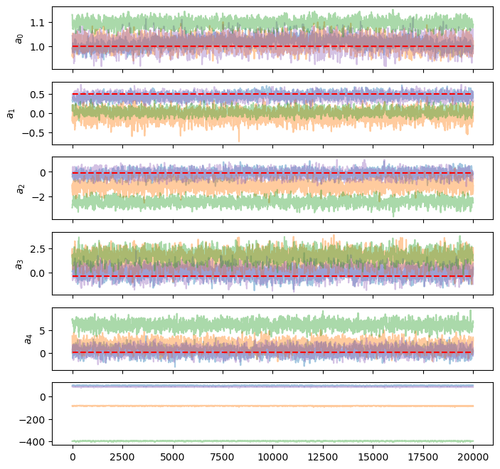
model = correct_model
fig, axes = plt.subplots(
    walkers["marginalized_sys_err"].model_sampler.chain.shape[1] + 1,
    1,
    figsize=(8, 8),
    sharex=True,
)
for i in range(walker.model_sampler.chain.shape[1]):
    # plot walkers
    for key, walker in walkers.items():
        axes[i].plot(walker.model_sampler.chain[:, i], alpha=0.4, color=colors[key])

    axes[i].set_ylabel(f"${model.params[i].latex_name}$")
    true_value = true_params[i]
    axes[i].hlines(true_value, 0, len(walker.model_sampler.chain), "r", linestyle="--")

# plot likelihoods
for key, walker in walkers.items():
    axes[-1].plot(walker.model_sampler.logp_chain, alpha=0.4, color=colors[key])

prior_samples = model_prior.rvs(walker.model_sampler.chain.shape[0])
prior_samples.shape

(20000, 5)

domain = np.zeros((len(walkers), correct_model.n_params, 2))
for i, (key, walker) in enumerate(walkers.items()):
    domain[i, ...] = np.array(
        [
            np.min(walker.model_sampler.chain, axis=0),
            np.max(walker.model_sampler.chain, axis=0),
        ]
    ).T
domain = np.array([np.min(domain[:, :, 0], axis=0), np.max(domain[..., 1], axis=0)])

domain.shape

(2, 5)

fig = plt.figure()
for key, walker in walkers.items():
    corner.corner(
        walker.model_sampler.chain,
        fig=fig,
        color=colors[key],
        range=domain.T,
        labels=[f"${p.latex_name}$" for p in correct_model.params],
        truths=true_params,
        labelpad=0.1,
        max_n_ticks=2,
        truth_color="k",
    )

    plt.plot([], [], color=colors[key], label=key)
fig.legend()
# plt.tight_layout()

<matplotlib.legend.Legend at 0x14a50aa62850>

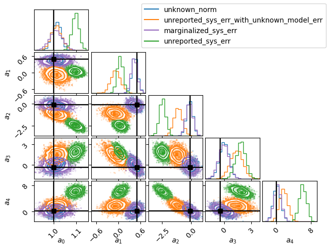
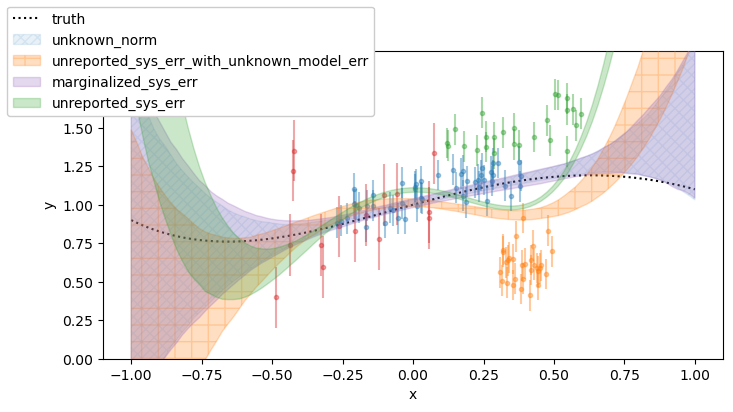
As expected, unknown_norm and marginalized_sys_err are the same. This is because they originate from the same exact statistical model, in which the normalization of each data set is a random variable. The latter explicitly marginalizes over the renormalization according to $\mathcal{N}(1,\sigma_{sys})$, whereas the former takes that distribution as a prior but attempts to learn the real distribution by conditioning the data.

In this case the underlying process for generating $N$ is exactly what the experimentalists report (that is, it is $\mathcal{N}(1,\sigma_{sys})$). If the experimentally reported $\sigma_{sys}$ was incorrect, then marginalized_sys_err would not be marginalizing over the correct distribution, and would converge to something wrong (try it!). On the other hand, with unknown_norm, incorrect experimentally reported $\sigma_{sys}$ just means a bad prior: $\sigma_{sys}$ doesn’t enter into the likelihood at all. Eventually, sampling should converge to the appropriate distribution.

Of course, the other two methods, which do not account for systematic error at all, fail to converge to the region of the truth.

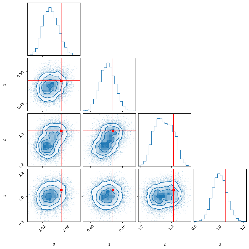
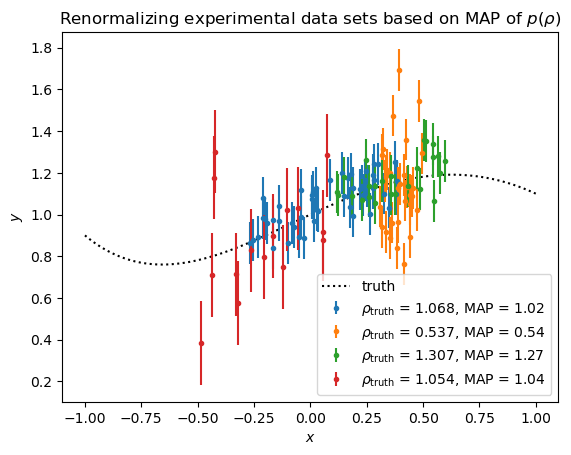
Let’s explore the performance of the inference of the normalizations from the “unknown norm” model

We will look at the posteriors of $\rho_i$, the renormalization of the model predictions with respect to each data set. We will look at the maxima a posteriori (MAP) and compare them to the values we actually renormalized by when generating the synthetic data. Then we will plot the experimental values renormalized by the MAP $\rho$s, and we should see that they re-align themselves with the truth.

norm_chain = np.array(
    [sampler.chain for sampler in walkers["unknown_norm"].likelihood_samplers]
)[:, :, 0]
norm_chain = np.exp(norm_chain.T)
norm_chain.shape

(20000, 4)

norm_log_posterior_vals = np.array(
    [sampler.logp_chain for sampler in walkers["unknown_norm"].likelihood_samplers]
).T
norm_log_posterior_vals.shape

(20000, 4)

map_idxs = np.argmax(norm_log_posterior_vals, axis=0)
N_data_sets = len(settings)
maps = norm_chain[map_idxs, np.arange(N_data_sets)]
maps

array([1.02222029, 0.5391869 , 1.26555557, 1.03850914])

np.array([obs.renormalization for obs in observations])

array([1.06789136, 0.53671203, 1.3071512 , 1.05429387])

np.mean(norm_chain, axis=0)

array([1.04122028, 0.52298738, 1.27509224, 1.00875858])

fig = corner.corner(
    norm_chain,
    labels=range(len(settings)),
    truths=[obs.renormalization for obs in observations],
    labelpad=0.1,
    max_n_ticks=2,
    color="tab:blue",
    truth_color="red",
)

plt.plot(truth.x, truth.y, "k:", label="truth")
for i, synthetic_observation in enumerate(observations):
    rho_hat = maps[i]
    plt.errorbar(
        synthetic_observation.x,
        synthetic_observation.y / rho_hat,
        np.sqrt(np.diag(synthetic_observation.statistical_covariance)),
        linestyle="none",
        marker=".",
        label=r"$\rho_{\text{truth}}$ = "
        + f"{synthetic_observation.renormalization:1.3f},"
        + r" MAP = "
        + f"{rho_hat:1.2f}",
    )
plt.xlabel("$x$")
plt.ylabel("$y$")
plt.legend()
plt.title(r"Renormalizing experimental data sets based on MAP of $p(\rho)$")

Text(0.5, 1.0, 'Renormalizing experimental data sets based on MAP of $p(\\rho)$')

predictive posteriors

walker.model_sampler.chain.shape

(20000, 5)

def predictive_post(chain, model, obs, n_samples, intervals):
    draw_idxs = rng.choice(np.arange(chain.shape[0]), n_samples)
    draws = chain[draw_idxs, :]
    ym = np.array([model(obs, *p) for p in draws])
    return np.percentile(ym, intervals, axis=0)

fig = plt.figure(figsize=(8, 4))
plt.plot(truth.x, truth.y, "k:", label="truth")

for synthetic_observation in observations:
    plt.errorbar(
        synthetic_observation.x,
        synthetic_observation.y,
        np.sqrt(np.diag(synthetic_observation.statistical_covariance)),
        linestyle="none",
        marker=".",
        alpha=0.4,
        # label=f"renormalization = {synthetic_observation.renormalization:1.3f}",
    )

hatches = ["//\\//\\", "|-", "", ""]
alphas = [0.1, 0.25, 0.25, 0.25]
for i, (key, walker) in enumerate(walkers.items()):
    intervals = predictive_post(
        walker.model_sampler.chain,
        correct_model,
        truth,
        1000,
        [16, 84],
    )
    plt.fill_between(
        truth.x,
        intervals[0],
        intervals[1],
        alpha=alphas[i],
        color=colors[key],
        label=key,
        hatch=hatches[i],
        zorder=99,
    )
plt.xlabel("x")
plt.ylabel("y")
plt.ylim([0, 2])
fig.legend(loc="upper left", framealpha=1)

<matplotlib.legend.Legend at 0x14a50a1d87d0>