30s optical potential calibration#
This notebook demonstrates a small end-to-end adaptive Metropolis calibration of an elastic differential cross section model using mock data .
import corner
import jitr
import matplotlib.pyplot as plt
import numpy as np
from jitr.optical_potentials.potential_forms import (
    thomas_safe,
    woods_saxon_prime_safe,
    woods_saxon_safe,
)
from scipy import stats

import rxmc
from rxmc.params import Parameter
Using database version X4-2025-12-31 located in: /mnt/home/beyerkyl/x4db/unpack_exfor-2025/X4-2025-12-31
Reaction and optical model#
Ca40 = (40, 20)
neutron = (1, 0)
E_lab = 14.1

rxn = jitr.reactions.ElasticReaction(target=Ca40, projectile=neutron)

mso = 1.0 / jitr.utils.constants.WAVENUMBER_PION


def central_potential(r, Vv, Wv, Rv, av, Wd, Rd, ad):
    return -(Vv + 1j * Wv) * woods_saxon_safe(r, Rv, av) + (
        4j * ad * Wd
    ) * woods_saxon_prime_safe(r, Rd, ad)


def spin_orbit_potential(r, Vso, Wso, Rso, aso):
    return (Vso + 1j * Wso) * mso**2 * thomas_safe(r, Rso, aso)


R = 1.2 * 40 ** (1 / 3)
fixed_spin_orbit = (6.0, -3, R, 0.45)


def extract_params(ws, *x):
    Vv, Wv, Rv, av, Wd, Rd, ad = x
    central_params = (Vv, Wv, Rv, av, Wd, Rd, ad)
    return central_params, fixed_spin_orbit


params = [
    Parameter("Vv", unit="MeV"),
    Parameter("Wv", unit="MeV"),
    Parameter("Rv", unit="fm"),
    Parameter("av", unit="fm"),
    Parameter("Wd", unit="MeV"),
    Parameter("Rd", unit="fm"),
    Parameter("ad", unit="fm"),
]

omp = rxmc.elastic_diffxs_model.ElasticDifferentialXSModel(
    "dXS/dA",
    interaction_central=central_potential,
    interaction_spin_orbit=spin_orbit_potential,
    calculate_interaction_from_params=extract_params,
    params=params,
    model_name="minimal_elastic_demo",
)
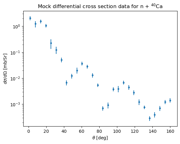
Generate mock data and construct the observation directly#
The key API change demonstrated here is that we can create an
ElasticDifferentialXSObservation directly from arrays and metadata, without
building an exfor_tools.Distribution object first.
angles_deg = np.linspace(2.0, 160.0, 28)
true_params = np.array(
    [48.0, 3.5, 1.1 * 40 ** (1 / 3), 0.7, 21, 1.2 * 40 ** (1 / 3), 0.5]
)

template_obs = rxmc.elastic_diffxs_observation.ElasticDifferentialXSObservation(
    x=angles_deg,
    y=np.ones_like(angles_deg, dtype=float),
    Elab=E_lab,
    reaction=rxn,
    quantity="dXS/dA",
    measurement_quantity="dXS/dA",
    y_units="barn / steradian",
    dataset_label="template",
)

y_true = omp.evaluate(template_obs, *true_params)

rng = np.random.default_rng(42)
y_stat_err = 0.2 * np.maximum(y_true, 1e-4)
y_mock = np.clip(y_true + rng.normal(scale=y_stat_err * 1.3), 1e-6, None)

obs = rxmc.elastic_diffxs_observation.ElasticDifferentialXSObservation(
    x=angles_deg,
    y=y_mock,
    Elab=E_lab,
    reaction=rxn,
    quantity="dXS/dA",
    measurement_quantity="dXS/dA",
    y_units="barn / steradian",
    y_stat_err=y_stat_err,
    dataset_label="mock elastic dataset",
)
plt.errorbar(np.rad2deg(obs.x), obs.y, obs.y_stat_err, linestyle="none", marker=".")
plt.xlabel(r"$\theta$ [deg]")
plt.ylabel(r"$d\sigma/d\Omega$ [mb/Sr]")
plt.yscale("log")
plt.title("Mock differential cross section data for n + $^{40}$Ca")
Text(0.5, 1.0, 'Mock differential cross section data for n + $^{40}$Ca')
Set up the inference problem#
constraint = rxmc.constraint.Constraint(
    observations=[obs],
    physical_model=omp,
    likelihood_model=rxmc.likelihood_model.LikelihoodModel(),
)
evidence = rxmc.evidence.Evidence(constraints=[constraint])

prior_mean = np.array(
    [50.0, 3, 1.2 * 40 ** (1 / 3), 0.65, 18, 1.2 * 40 ** (1 / 3), 0.65]
)
prior_cov = np.diag([7, 7, 0.2, 0.2, 10, 0.2, 0.2]) ** 2
prior = stats.multivariate_normal(mean=prior_mean, cov=prior_cov)

walker = rxmc.walker.Walker(
    model_sampler=rxmc.param_sampling.BatchedAdaptiveMetropolisSampler(
        params=omp.params,
        prior=prior,
        starting_location=prior_mean,
        initial_proposal_cov=prior_cov / 100,
    ),
    evidence=evidence,
    rng=np.random.default_rng(7),
)
%%time
walker.walk(n_steps=20000, burnin=1000, batch_size=1000, verbose=True)
samples = walker.model_sampler.chain[40:]
acceptance_fraction = walker.model_sampler.overall_acceptance_fraction()
acceptance_fraction
Burn-in batch 1/1 completed, 1000 steps.
Batch: 1/20 completed, 1000 steps.
  Model parameter acceptance fraction: 0.172
Batch: 2/20 completed, 1000 steps.
  Model parameter acceptance fraction: 0.181
Batch: 3/20 completed, 1000 steps.
  Model parameter acceptance fraction: 0.199
Batch: 4/20 completed, 1000 steps.
  Model parameter acceptance fraction: 0.202
Batch: 5/20 completed, 1000 steps.
  Model parameter acceptance fraction: 0.212
Batch: 6/20 completed, 1000 steps.
  Model parameter acceptance fraction: 0.269
Batch: 7/20 completed, 1000 steps.
  Model parameter acceptance fraction: 0.250
Batch: 8/20 completed, 1000 steps.
  Model parameter acceptance fraction: 0.210
Batch: 9/20 completed, 1000 steps.
  Model parameter acceptance fraction: 0.203
Batch: 10/20 completed, 1000 steps.
  Model parameter acceptance fraction: 0.181
Batch: 11/20 completed, 1000 steps.
  Model parameter acceptance fraction: 0.225
Batch: 12/20 completed, 1000 steps.
  Model parameter acceptance fraction: 0.220
Batch: 13/20 completed, 1000 steps.
  Model parameter acceptance fraction: 0.172
Batch: 14/20 completed, 1000 steps.
  Model parameter acceptance fraction: 0.243
Batch: 15/20 completed, 1000 steps.
  Model parameter acceptance fraction: 0.147
Batch: 16/20 completed, 1000 steps.
  Model parameter acceptance fraction: 0.222
Batch: 17/20 completed, 1000 steps.
  Model parameter acceptance fraction: 0.211
Batch: 18/20 completed, 1000 steps.
  Model parameter acceptance fraction: 0.161
Batch: 19/20 completed, 1000 steps.
  Model parameter acceptance fraction: 0.218
Batch: 20/20 completed, 1000 steps.
  Model parameter acceptance fraction: 0.209
CPU times: user 36.4 s, sys: 15 ms, total: 36.4 s
Wall time: 36.4 s
0.20535
Posterior summary and predictive band#
posterior_mean = np.mean(samples, axis=0)
posterior_std = np.std(samples, axis=0)
draw_indices = np.linspace(
    0, samples.shape[0] - 1, min(60, samples.shape[0]), dtype=int
)
posterior_draws = samples[draw_indices]
y_draws = np.array(
    [omp.visualizable_model_prediction(obs, *draw) for draw in posterior_draws]
)
y_mean = np.mean(y_draws, axis=0)
y_low, y_high = np.percentile(y_draws, [5, 95], axis=0)
y_true = omp.visualizable_model_prediction(obs, *true_params)
for i in range(len(params)):
    print(
        f"{params[i].name}: truth={true_params[i]:1.2f} mean={posterior_mean[i]:1.2f}, std={posterior_std[i]:1.2f}"
    )
Vv: truth=48.00 mean=43.94, std=2.62
Wv: truth=3.50 mean=4.73, std=2.03
Rv: truth=3.76 mean=3.93, std=0.15
av: truth=0.70 mean=0.64, std=0.05
Wd: truth=21.00 mean=18.74, std=2.93
Rd: truth=4.10 mean=4.10, std=0.08
ad: truth=0.50 mean=0.50, std=0.05
fig, axes = plt.subplots(samples.shape[1] + 1, 1, figsize=(8, 8), sharex=True)
logp = walker.model_sampler.logp_chain
for i in range(samples.shape[1]):
    axes[i].plot(samples[:, i])
    axes[i].set_ylabel(f"${omp.params[i].latex_name}$ [{omp.params[i].unit}]")
    true_value = true_params[i]
    axes[i].hlines(true_value, 0, len(samples), "r", linestyle="--")
axes[-1].plot(logp)
axes[-1].set_ylabel(r"$\log{\mathcal{L}(\alpha_i | \mathcal{O})}$")

axes[-1].set_xlabel(r"$i$")
Text(0.5, 0, '$i$')
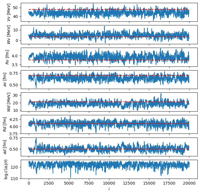
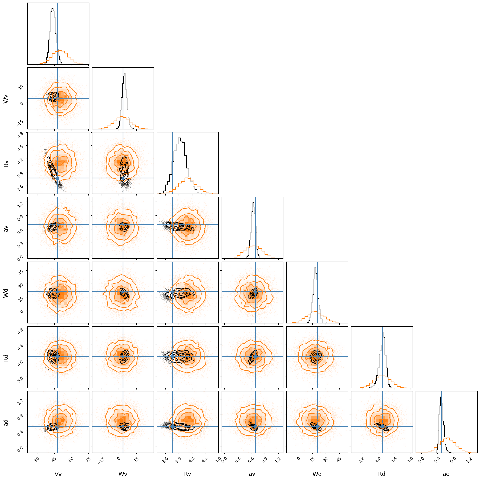
fig = corner.corner(
    samples,
    labels=[p.name for p in omp.params],
    truths=true_params,
    label_kwargs={"fontsize": 14},
)
_ = corner.corner(prior.rvs(5000), fig=fig, color="tab:orange")
fig, ax = plt.subplots(1, 1, figsize=(8, 4))

angles_plot = np.rad2deg(obs.visualization_workspace.angles)
ax.errorbar(np.rad2deg(obs.x), obs.y, yerr=obs.y_stat_err, fmt="o", label="Mock data")
ax.plot(angles_plot, y_true, label="Truth", linewidth=2, alpha=0.8)
ax.fill_between(
    angles_plot, y_low, y_high, alpha=0.4, label="90% predictive posterior band"
)
ax.set_xlabel("Angle (deg)")
ax.set_ylabel("d$\\sigma$/d$\\Omega$ (b/sr)")
ax.legend()
ax.set_yscale("log")
fig.tight_layout()
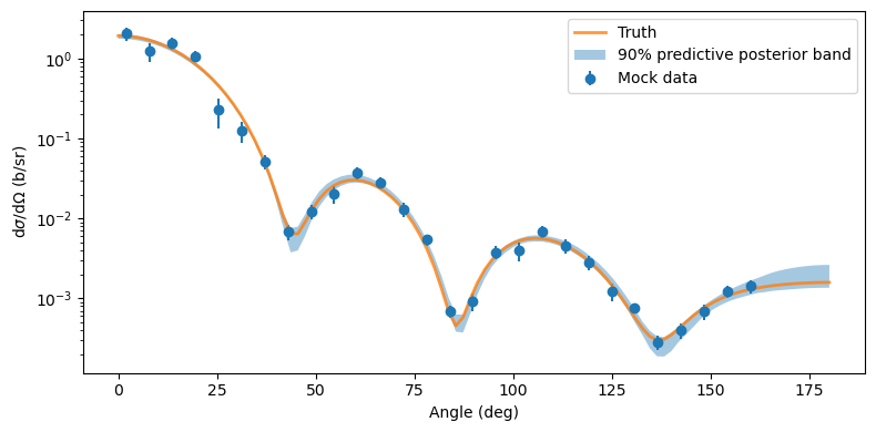
Note that the predictive posterior has excellent coverage of the training data, even though the parameter inference was not perfect. One must be wary of infering parameters from optical potentials, as multiple different sets of parameter values can produce the same cross section!