Yamaguchi scattering example

This notebook shows how to use the spectral solver on the classic Yamaguchi non-local potential.

We will:

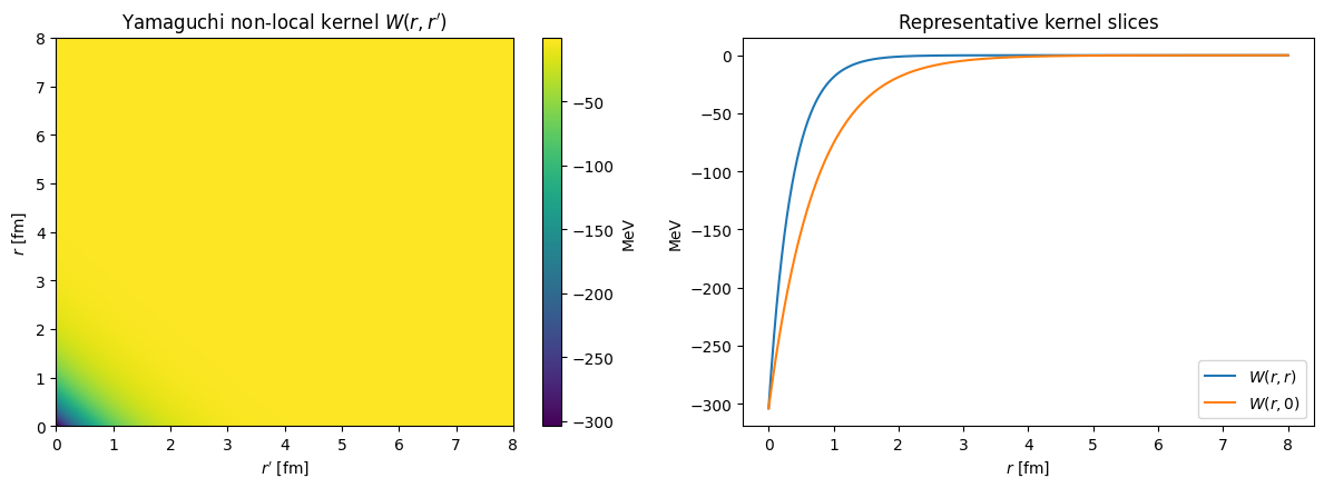
1. visualize the non-local kernel itself,

2. evaluate phase shifts on a fine energy grid from the spectrum,

3. compare the l = 0 phase shift against the closed-form separable-model result,

from __future__ import annotations

import jax.numpy as jnp
import matplotlib.pyplot as plt
import numpy as np

import lax as lm

HBAR2_2MU = lm.constants.hbar2_over_2mu(1.008665, 1.008665)  # MeV·fm²
ALPHA = 0.2316053
BETA = 1.3918324

def yamaguchi_kernel(r1: jax.Array, r2: jax.Array) -> jax.Array:
    return -2.0 * BETA * (ALPHA + BETA) ** 2 * jnp.exp(-BETA * (r1 + r2)) * HBAR2_2MU


def yamaguchi_s_wave_analytic_phase_deg(energies_mev: np.ndarray) -> np.ndarray:
    k = np.sqrt(energies_mev / HBAR2_2MU)
    numerator = 2.0 * BETA * (ALPHA + BETA) ** 2 * k
    denominator = (BETA**2 + k**2) ** 2 - (ALPHA + BETA) ** 2 * (BETA**2 - k**2)
    return np.degrees(np.arctan2(numerator, denominator))


def unwrap_phase_shift_deg(phase_deg: np.ndarray) -> np.ndarray:
    return np.degrees(np.unwrap(2.0 * np.radians(phase_deg))) / 2.0

r_plot = np.linspace(0.0, 8.0, 200)
r1_grid, r2_grid = np.meshgrid(r_plot, r_plot, indexing="ij")
kernel_values = np.asarray(yamaguchi_kernel(jnp.asarray(r1_grid), jnp.asarray(r2_grid)))

fig, axes = plt.subplots(1, 2, figsize=(12, 4.5))
image = axes[0].imshow(
    kernel_values,
    extent=[r_plot[0], r_plot[-1], r_plot[0], r_plot[-1]],
    origin="lower",
    aspect="auto",
    cmap="viridis",
)
axes[0].set_title("Yamaguchi non-local kernel $W(r, r')$")
axes[0].set_xlabel(r"$r'$ [fm]")
axes[0].set_ylabel(r"$r$ [fm]")
fig.colorbar(image, ax=axes[0], label="MeV")

axes[1].plot(r_plot, np.diag(kernel_values), label=r"$W(r, r)$")
axes[1].plot(r_plot, kernel_values[:, 0], label=r"$W(r, 0)$")
axes[1].set_title("Representative kernel slices")
axes[1].set_xlabel(r"$r$ [fm]")
axes[1].set_ylabel("MeV")
axes[1].legend()
fig.tight_layout()

Compile the solver

def yamaguchi_solver(partial_waves: list[int], energies: jax.Array) -> lm.Solver:
    # One solver batches all partial waves: each ℓ is an independent symmetry
    # block (the N_c = 1 case of DESIGN.md §15.5), solved in one vmapped call
    # instead of one compiled solver per ℓ.
    return lm.compile(
        mesh=lm.MeshSpec("legendre", "x", n=20, scale=15.0),
        blocks=[
            [lm.ChannelSpec(l=ell, threshold=0.0, mass_factor=HBAR2_2MU)]
            for ell in partial_waves
        ],
        operators=("T+L",),
        solvers=("spectrum", "phases"),
        energies=energies,
    )

%%time
energies = jnp.linspace(0.05, 10.0, 100)
partial_waves = list(range(10))

solver = yamaguchi_solver(partial_waves, energies)

CPU times: user 790 ms, sys: 14.1 ms, total: 804 ms
Wall time: 788 ms

Evaluate the interaction matrix

solver.nonlocal_potential (and its local counterpart solver.local_potential) automatically cast an interaction kernel across all the energies and symmetry blocks built into the solver. In this case, the potential is not energy or partial wave dependent.

%%time
potential = solver.nonlocal_potential(yamaguchi_kernel)
print(f"potential is an {type(potential)}. It has shape {potential.block.shape}")

potential is an <class 'lax.types.Interaction'>. It has shape (20, 20)
CPU times: user 326 ms, sys: 3.1 ms, total: 329 ms
Wall time: 326 ms

Solve the system

solver.spectrum performs an eigendecomposition of the Bloch-Hamiltonian. Note that the first time this is run, the JIT compilation will take place. Run it again to get the accurate result.

%%time
spectrum = solver.spectrum(potential)

CPU times: user 162 ms, sys: 17 ms, total: 179 ms
Wall time: 144 ms

Calculate of phase shifts from the resulting eigendecomposition

The \(\mathcal{R}\)-matrix is expanded using the eigendecomposition stored in spectrum. The boundary conditions baked into solver thus allows for the calculation of \(\mathcal{S}\)-matrix elements and phase shifts from the \(\mathcal{R}\)-matrix.

%%time
phases_deg = np.degrees(np.asarray(solver.phases(spectrum)[:, :, 0]))  # (N_b, N_E)
phase_curves = {
    ell: unwrap_phase_shift_deg(row)
    for ell, row in zip(partial_waves, phases_deg, strict=True)
}

CPU times: user 1.3 s, sys: 37.7 ms, total: 1.34 s
Wall time: 412 ms

analytic_s_wave = yamaguchi_s_wave_analytic_phase_deg(np.asarray(energies))

# The phase shift is only defined modulo 180°, so align the unwrapped mesh
# curve with the analytic branch before comparing.
branch_shift = 180.0 * np.round(np.mean(analytic_s_wave - phase_curves[0]) / 180.0)
phase_curves[0] = phase_curves[0] + branch_shift
max_s_wave_error = np.max(np.abs(phase_curves[0] - analytic_s_wave))
print(
    f"Maximum |δ_mesh - δ_analytic| for l=0 on this grid: {max_s_wave_error:.3e} degrees"
)

Maximum |δ_mesh - δ_analytic| for l=0 on this grid: 6.318e-07 degrees

fig, axes = plt.subplots(1, 2, figsize=(13, 4.8))

axes[0].plot(
    np.asarray(energies), analytic_s_wave, label="analytic s-wave", linewidth=2.5
)
axes[0].plot(
    np.asarray(energies), phase_curves[0], "--", label="spectral s-wave", linewidth=2.0
)
axes[0].set_title(r"Yamaguchi $\ell=0$ phase shift")
axes[0].set_xlabel("Energy [MeV]")
axes[0].set_ylabel("Phase shift [deg]")
axes[0].legend()

for angular_momentum in partial_waves:
    axes[1].plot(
        np.asarray(energies),
        phase_curves[angular_momentum],
        label=rf"$\ell={angular_momentum}$",
    )
axes[1].set_title("Several partial waves from the spectral solver")
axes[1].set_xlabel("Energy [MeV]")
axes[1].set_ylabel("Phase shift [deg]")
axes[1].legend()
fig.tight_layout()

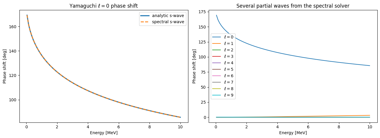
The Yamaguchi kernel is rank-one and separable, so the l = 0 channel has a closed-form phase-shift curve. That makes it a good analytic check on the spectral solver. The phase shift is only defined modulo \(180^\circ\), so the notebook unwraps \(2\delta\) and aligns the branch with the analytic curve before comparing — the remaining difference is pure mesh error. The higher partial waves shown here are still useful numerically, even though the simplest closed-form comparison is the s-wave one.