α + \(^{208}\)Pb optical-model example

This notebook walks through the single-channel optical-model benchmark from Descouvemont’s CPC paper.

We will:

1. define the optical Woods-Saxon + Coulomb potential,

2. visualize its real, imaginary, and Coulomb pieces,

3. evaluate the collision-matrix element for the benchmark energies,

4. compare all three validated solver paths:

   • real spectrum path (eigh)

   • complex spectrum path (eig)

   • complex direct path (linear_solve / rmatrix_direct)

5. compare the complex results against Descouvemont Appendix A.

from __future__ import annotations

import jax.numpy as jnp
import matplotlib.pyplot as plt
import numpy as np

import lax as lm
from lax.boundary import BoundaryValues

OPTICAL_ENERGIES = np.array([10.0, 20.0, 30.0, 40.0, 50.0], dtype=np.float64)
APPENDIX_A_S = np.array(
    [
        1.0000e00 + 5.9801e-19j,
        1.0000e00 + 7.4950e-07j,
        9.9893e-01 + 9.0496e-03j,
        6.5081e-01 + 2.9560e-01j,
        6.4367e-02 + 4.1130e-02j,
    ],
    dtype=np.complex128,
)
ALPHA_PB_MASS_FACTOR = lm.constants.hbar2_over_2mu(
    4.001506, 207.9767
)  # α + ²⁰⁸Pb  MeV·fm²
BENCHMARK_L = 20
CHANNEL_RADIUS = 14.0


def unwrap_phase_shift_deg(phase_deg: np.ndarray) -> np.ndarray:
    # δ is only defined modulo 180°: unwrap 2δ to remove branch jumps.
    return np.degrees(np.unwrap(2.0 * np.radians(phase_deg))) / 2.0


def optical_potential_parts(
    r: jnp.ndarray, imag_depth: float
) -> tuple[jnp.ndarray, jnp.ndarray, jnp.ndarray, jnp.ndarray]:
    v0 = 100.0
    radius = 1.1132 * (208.0 ** (1.0 / 3.0) + 4.0 ** (1.0 / 3.0))
    diffuseness = 0.5803
    woods_saxon = 1.0 / (1.0 + jnp.exp((r - radius) / diffuseness))
    nuclear_real = -v0 * woods_saxon
    nuclear_imag = -imag_depth * woods_saxon
    coulomb = 2.0 * 82.0 * 1.44 / r
    total = nuclear_real + coulomb + 1.0j * nuclear_imag
    return total, nuclear_real, nuclear_imag, coulomb


def optical_potential(r: jnp.ndarray, imag_depth: float) -> jnp.ndarray:
    total, _, _, _ = optical_potential_parts(r, imag_depth)
    return total


def complex_solver(method: str, solvers: tuple[str, ...]) -> lm.Solver:
    return lm.compile(
        mesh=lm.MeshSpec("legendre", "x", n=60, scale=CHANNEL_RADIUS),
        channels=(
            lm.ChannelSpec(
                l=BENCHMARK_L, threshold=0.0, mass_factor=ALPHA_PB_MASS_FACTOR
            ),
        ),
        operators=("T+L",),
        solvers=solvers,
        energies=OPTICAL_ENERGIES,
        V_is_complex=True,
        method=method,
        z1z2=(2, 82),
    )


def real_solver(method: str, solvers: tuple[str, ...]) -> lm.Solver:
    return lm.compile(
        mesh=lm.MeshSpec("legendre", "x", n=60, scale=CHANNEL_RADIUS),
        channels=(
            lm.ChannelSpec(
                l=BENCHMARK_L, threshold=0.0, mass_factor=ALPHA_PB_MASS_FACTOR
            ),
        ),
        operators=("T+L",),
        solvers=solvers,
        energies=OPTICAL_ENERGIES,
        method=method,
        z1z2=(2, 82),
    )


def smatrix_from_direct_rmatrix(
    solver: lm.Solver, potential: jnp.ndarray
) -> np.ndarray:
    assert solver.rmatrix_direct is not None
    assert solver.boundary is not None
    r_values = solver.rmatrix_direct(potential)
    smatrices = []
    for energy_index in range(r_values.shape[0]):
        boundary = BoundaryValues(
            H_plus=solver.boundary.H_plus[energy_index],
            H_minus=solver.boundary.H_minus[energy_index],
            H_plus_p=solver.boundary.H_plus_p[energy_index],
            H_minus_p=solver.boundary.H_minus_p[energy_index],
            is_open=solver.boundary.is_open[energy_index],
            k=solver.boundary.k[energy_index],
        )
        smatrix = lm.spectral.smatrix_from_R(r_values[energy_index], boundary)
        smatrices.append(np.asarray(smatrix))
    return np.stack(smatrices)

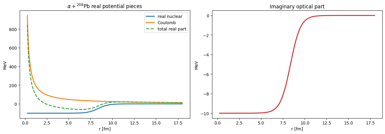
Potential shape

The benchmark potential combines a real Woods-Saxon attraction, an imaginary absorptive Woods-Saxon part, and a point-Coulomb term. The complex optical calculation uses an imaginary depth of 10 MeV.

r_plot = np.linspace(0.25, 18.0, 500)
total, nuclear_real, nuclear_imag, coulomb = optical_potential_parts(
    jnp.asarray(r_plot), imag_depth=10.0
)

fig, axes = plt.subplots(1, 2, figsize=(13, 4.6))
axes[0].plot(r_plot, np.asarray(nuclear_real), label="real nuclear", linewidth=2.2)
axes[0].plot(r_plot, np.asarray(coulomb), label="Coulomb", linewidth=2.2)
axes[0].plot(
    r_plot, np.asarray(total.real), "--", label="total real part", linewidth=2.0
)
axes[0].set_title(r"$\alpha + {}^{208}\mathrm{Pb}$ real potential pieces")
axes[0].set_xlabel("r [fm]")
axes[0].set_ylabel("MeV")
axes[0].legend()

axes[1].plot(r_plot, np.asarray(nuclear_imag), color="tab:red", linewidth=2.2)
axes[1].set_title("Imaginary optical part")
axes[1].set_xlabel("r [fm]")
axes[1].set_ylabel("MeV")

fig.tight_layout()

Three solver paths on the same benchmark

The validated test suite checks three related calculations:

• a real-potential spectrum path using eigh,

• a complex spectrum path using eig,

• a complex direct path using linear_solve and rmatrix_direct.

The complex eig and direct paths should both reproduce the published Appendix A collision-matrix values, and the real-potential eigh path provides a clean Hermitian reference limit.

solver_real = real_solver("eigh", ("spectrum", "smatrix"))
solver_complex_eig = complex_solver("eig", ("spectrum", "smatrix"))
solver_complex_direct = complex_solver("linear_solve", ("rmatrix_direct",))

potential_real = solver_real.local_potential(
    lambda r: jnp.real(optical_potential(r, imag_depth=0.0))
)
potential_complex_eig = solver_complex_eig.local_potential(
    lambda r: optical_potential(r, imag_depth=10.0)
)
potential_complex_direct = solver_complex_direct.local_potential(
    lambda r: optical_potential(r, imag_depth=10.0)
)

smatrix_real = np.asarray(solver_real.smatrix(solver_real.spectrum(potential_real)))[
    :, 0, 0
]
smatrix_complex_eig = np.asarray(
    solver_complex_eig.smatrix(solver_complex_eig.spectrum(potential_complex_eig))
)[:, 0, 0]
smatrix_complex_direct = smatrix_from_direct_rmatrix(
    solver_complex_direct, potential_complex_direct
)[:, 0, 0]

print("Energy   Appendix A S(E)               eig S(E)                     direct S(E)")
for energy, appendix_value, eig_value, direct_value in zip(
    OPTICAL_ENERGIES,
    APPENDIX_A_S,
    smatrix_complex_eig,
    smatrix_complex_direct,
):
    print(
        f"{energy:5.1f}   {appendix_value.real: .6f}{appendix_value.imag:+.6f}j   "
        f"{eig_value.real: .6f}{eig_value.imag:+.6f}j   "
        f"{direct_value.real: .6f}{direct_value.imag:+.6f}j"
    )

print()
print(
    f"max |eig - Appendix A|    = {np.max(np.abs(smatrix_complex_eig - APPENDIX_A_S)):.3e}"
)
print(
    f"max |direct - Appendix A| = {np.max(np.abs(smatrix_complex_direct - APPENDIX_A_S)):.3e}"
)
print(
    f"max |eig - direct|        = {np.max(np.abs(smatrix_complex_eig - smatrix_complex_direct)):.3e}"
)

Energy   Appendix A S(E)               eig S(E)                     direct S(E)
 10.0    1.000000+0.000000j    1.000000+0.000000j    1.000000+0.000000j
 20.0    1.000000+0.000001j    1.000000+0.000001j    1.000000+0.000001j
 30.0    0.998930+0.009050j    0.998997+0.008447j    0.998997+0.008447j
 40.0    0.650810+0.295600j    0.667031+0.297554j    0.667031+0.297554j
 50.0    0.064367+0.041130j    0.080249+0.044620j    0.080249+0.044620j

max |eig - Appendix A|    = 1.634e-02
max |direct - Appendix A| = 1.634e-02
max |eig - direct|        = 1.775e-12

fig, axes = plt.subplots(1, 2, figsize=(13, 4.8))

axes[0].plot(
    OPTICAL_ENERGIES, APPENDIX_A_S.real, "o-", label="Appendix A real", linewidth=2.2
)
axes[0].plot(
    OPTICAL_ENERGIES, smatrix_complex_eig.real, "--", label="eig real", linewidth=2.0
)
axes[0].plot(
    OPTICAL_ENERGIES,
    smatrix_complex_direct.real,
    ":",
    label="direct real",
    linewidth=2.0,
)
axes[0].plot(
    OPTICAL_ENERGIES, APPENDIX_A_S.imag, "o-", label="Appendix A imag", linewidth=2.2
)
axes[0].plot(
    OPTICAL_ENERGIES, smatrix_complex_eig.imag, "--", label="eig imag", linewidth=2.0
)
axes[0].plot(
    OPTICAL_ENERGIES,
    smatrix_complex_direct.imag,
    ":",
    label="direct imag",
    linewidth=2.0,
)
axes[0].set_title("Complex optical benchmark vs Appendix A")
axes[0].set_xlabel("Energy [MeV]")
axes[0].set_ylabel(r"$S_{20}(E)$")
axes[0].legend(ncol=2, fontsize=9)

axes[1].plot(
    OPTICAL_ENERGIES,
    np.abs(smatrix_real),
    marker="o",
    label="real spectrum |S|",
    linewidth=2.2,
)
axes[1].plot(
    OPTICAL_ENERGIES,
    np.abs(smatrix_complex_eig),
    marker="s",
    label="complex eig |S|",
    linewidth=2.0,
)
axes[1].plot(
    OPTICAL_ENERGIES,
    np.abs(smatrix_complex_direct),
    marker="^",
    label="complex direct |S|",
    linewidth=2.0,
)
axes[1].set_title("Magnitude across the three validated paths")
axes[1].set_xlabel("Energy [MeV]")
axes[1].set_ylabel(r"$|S_{20}(E)|$")
axes[1].legend()

fig.tight_layout()

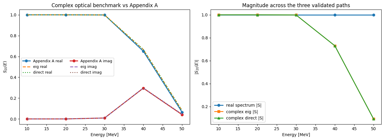
The two complex methods track each other closely because they are evaluating the same physical optical-model problem through different numerical routes. The eig path uses the complex spectrum of the Bloch-augmented Hamiltonian, while the direct path evaluates the R-matrix with explicit linear solves at each energy. The real eigh path is included because it is the Hermitian limit of the same benchmark setup and provides a useful baseline for how the optical absorption changes the collision-matrix magnitude.

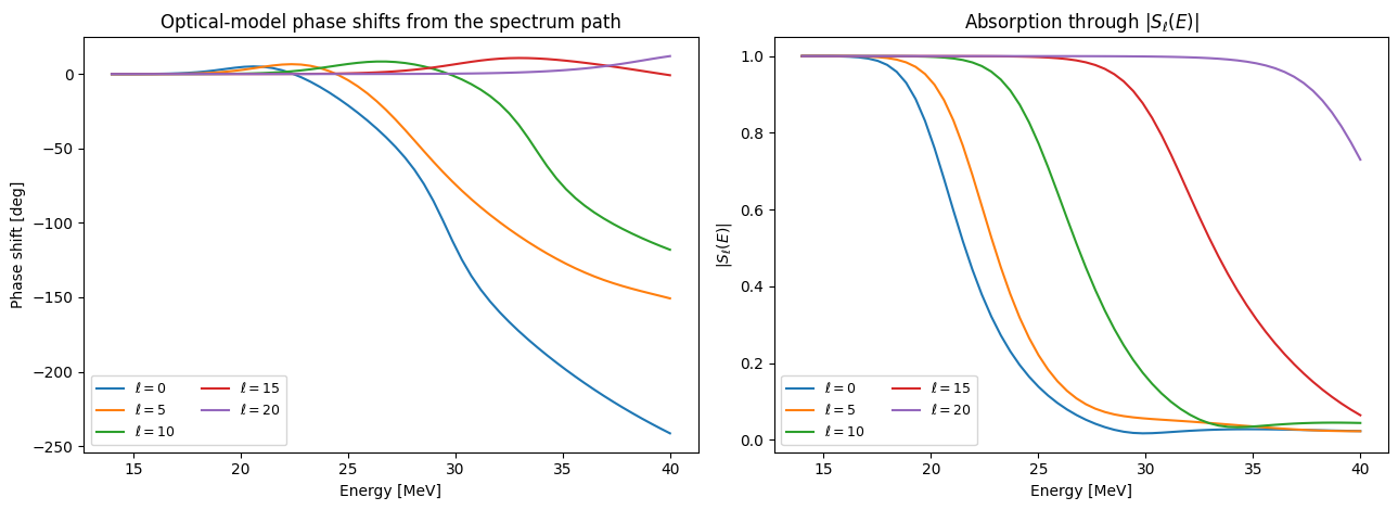
Phase shifts across several partial waves

The single benchmark channel uses l = 20, but the same optical potential can be scanned across many partial waves. Each partial wave is an independent symmetry block (the N_c = 1 case of blocks=), so one compile batches all of them on a leading axis instead of building one solver per wave. The expensive part here is the compile step, because it precomputes Coulomb boundary values across the full energy grid with mpmath. To make that cost visible, the scan is split into separate timed compile and solve cells.

%%time
fine_energies = jnp.linspace(14.0, 40.0, 60)
partial_waves = [0, 5, 10, 15, 20]
# One compile bakes the per-ℓ Coulomb boundary values and batches all five
# waves as symmetry blocks on a leading (N_b,) axis (DESIGN.md §15.5).
solver_pw = lm.compile(
    mesh=lm.MeshSpec("legendre", "x", n=60, scale=CHANNEL_RADIUS),
    blocks=[
        [lm.ChannelSpec(l=ell, threshold=0.0, mass_factor=ALPHA_PB_MASS_FACTOR)]
        for ell in partial_waves
    ],
    operators=("T+L",),
    solvers=("spectrum", "smatrix", "phases"),
    energies=fine_energies,
    V_is_complex=True,
    method="eig",
    z1z2=(2, 82),
)

CPU times: user 3min 21s, sys: 46.6 ms, total: 3min 21s
Wall time: 3min 33s

%%time
potential = solver_pw.local_potential(lambda r: optical_potential(r, imag_depth=10.0))
spectrum = solver_pw.spectrum(potential)  # one batched call over all partial waves
phases_deg = np.degrees(np.asarray(solver_pw.phases(spectrum)[:, :, 0]))  # (N_b, N_E)
abs_s = np.abs(np.asarray(solver_pw.smatrix(spectrum)[:, :, 0, 0]))  # (N_b, N_E)
phase_curves = {
    ell: unwrap_phase_shift_deg(row)
    for ell, row in zip(partial_waves, phases_deg, strict=True)
}
abs_s_curves = dict(zip(partial_waves, abs_s, strict=True))

CPU times: user 3.66 s, sys: 50 ms, total: 3.71 s
Wall time: 989 ms

fig, axes = plt.subplots(1, 2, figsize=(13, 4.8))
for angular_momentum in partial_waves:
    axes[0].plot(
        np.asarray(fine_energies),
        phase_curves[angular_momentum],
        label=rf"$\ell={angular_momentum}$",
    )
    axes[1].plot(
        np.asarray(fine_energies),
        abs_s_curves[angular_momentum],
        label=rf"$\ell={angular_momentum}$",
    )

axes[0].set_title("Optical-model phase shifts from the spectrum path")
axes[0].set_xlabel("Energy [MeV]")
axes[0].set_ylabel("Phase shift [deg]")
axes[0].legend(ncol=2, fontsize=9)

axes[1].set_title(r"Absorption through $|S_\ell(E)|$")
axes[1].set_xlabel("Energy [MeV]")
axes[1].set_ylabel(r"$|S_\ell(E)|$")
axes[1].legend(ncol=2, fontsize=9)

fig.tight_layout()